Continuous Distributions

This page describes the architecture of ProvSQL’s continuous random-variable surface: the on-disk gates, the per-family Distribution class hierarchy and its rule registries, the SQL composite type, the planner-hook rewriter’s classifier, the Monte Carlo sampler, the RangeCheck / AnalyticEvaluator / Expectation chain, the HybridEvaluator’s simplifier and island decomposer, the conditional-inference path, the aggregate dispatch, and the Studio rendering hooks. The user-facing description lives in Continuous Distributions.

Gate Types

Four gate types described below back the continuous surface, plus the gate_observe evidence gate covered in Latent variables further down; all are appended to the gate_type enum in provsql_utils.h before the gate_invalid sentinel, with no renumbering of the existing values. The companion provenance_gate SQL enum in sql/provsql.common.sql mirrors the C enum identically. (The conditioning marker gate_conditioned is shared with the Boolean surface and described in Probability Evaluation; its interaction with the moment evaluators is covered in Conditional Evaluation below.)

gate_rv

Random-variable leaf. The gate’s extra blob carries the distribution as text, <family>:<p1>[,<p2>] – e.g. "normal:2.5,0.5" for normal(2.5, 0.5) or "exponential:2" for exponential(2). The family token is not an enum: it is resolved at parse time against the distribution registry (see The Distribution Class Hierarchy below), so the set of valid blobs grows with the registered families – currently normal, uniform, exponential, erlang, gamma, lognormal, weibull, pareto, beta, logistic, inverse_gamma, inverse_gaussian, plus the discrete count families poisson, binomial, geometric, negative_binomial (whose blobs appear as gate_rv leaves only in the parametric/latent form – see Latent variables below).

Categorical random variables share no gate_rv encoding; they are encoded as a block of gate_mulinput gates under a gate_mixture (see below). The literal discrete count constructors (Poisson, Binomial, …) are SQL-level constructors over that categorical encoding, not gate types.

gate_arith

N-ary arithmetic over scalar children. The operator tag lives in info1 of the gate’s GateInformation: provsql_arith_op is PLUS = 0, TIMES = 1, MINUS = 2, DIV = 3, NEG = 4, MAX = 5, MIN = 6, POW = 7, LN = 8, EXP = 9, PERCENTILE = 10 (the percentile_cont order statistic, see Statistic aggregates below). MAX / MIN are the n-ary order statistics behind greatest / least and the max / min aggregates. POW (binary, real branch only) and LN carry evaluation-time domain guards (see the sampler section); EXP is total. The enum is append-only: the values are persisted on disk and must not be renumbered.

gate_mixture

Probabilistic mixture. The wire vector is [p, x, y] for a Bernoulli mixture (with p a Boolean gate and x, y scalar RV roots) or [key, mul_1, …, mul_n] for a categorical block (with key a fresh gate_input anchoring the block and each mul_i a gate_mulinput carrying the outcome value in its extra and its probability via set_prob).

gate_case

N-ary guarded selection over scalar children, with first-match semantics: the wire vector is [guard_1, value_1, …, guard_k, value_k, default] (odd length 2k + 1), and the gate’s value is the value_i of the first guard (a Boolean event, typically a gate_cmp) that holds, else the default. It carries data only in its wires – no info / extra, following the gate_conditioned precedent. Minted by provenance_case (and its random_variable wrapper rv_case), the target of the planner hook’s lowering of SQL CASE over random_variable branches. It is a real arm in the MC sampler, in RangeCheck (support = union of the value branches), and in the Expectation evaluator (closed-form moments via the guard-partition integrator below, Monte Carlo otherwise); like every measure-carrier gate it is refused by the general sr_* semirings (a guarded selection is not a semiring operation).

In addition, gate_value gains a float8 mode: the extra blob is parsed as a double by the RV evaluators (parseDoubleStrict in the MC sampler, extract_finite_double in RangeCheck), coexisting with having_semantics.cpp’s string-based extract_constant_string path, so gate_value covers both the deterministic mode used in HAVING sub-circuits and the random-variable-constant mode used by as_random.

The Distribution Class Hierarchy

src/distributions/ holds the per-family class hierarchy that every evaluator dispatches through; no evaluator names a family. The abstract interface is distributions/Distribution.h; the registries live in distributions/Distribution.cpp; each family is one self-contained implementation file (normal.cpp, uniform.cpp, exponential.cpp, erlang.cpp, gamma.cpp, lognormal.cpp, weibull.cpp, pareto.cpp, beta.cpp, logistic.cpp, inverse_gamma.cpp, inverse_gaussian.cpp, and the discrete poisson.cpp, binomial.cpp, geometric.cpp, negative_binomial.cpp) sharing only the internal header DistributionCommon.h. The logistic family is the location-scale logistic(μ, s) whose CDF is the logistic sigmoid $F(x) = \sigma((x - \mu)/s)$ and whose quantile is the logit $\mu + s\,\ln(p/(1-p))$ , so it realises the logit-link selection noise exactly; its mean is affine in μ (meanIsAffine).

A Distribution is a transient per-family view constructed from a parsed spec by makeDistribution. Its interface groups into:

identity: family() returns the interned DistributionFamily descriptor (name token, parameter count, display label, parameter symbols, factory) – descriptor-pointer equality is family identity; there is no family enum anywhere;
closed-form moments: mean(), variance(), rawMoment(k), plus the optional truncatedRawMoment(lo, hi, k) and iidOrderStatMean(n, isMax);
density / distribution: pdf(x), cdf(x) – a family that has no closed form returns NaN (the NaN-as-undecided contract: callers treat NaN as “fall back”, never as a value); the optional quantile(p) returns nullopt when there is no elementary inverse;
ranges: support(), integrationRange() (a finite quadrature window), plotRange() (for Studio’s density previews);
sampling: sample(rng), plus the optional sampleTruncated(rng, lo, hi, n) for rejection-free conditioned draws;
structure: affine(a, b) (the family’s image under a·X + b, or nullptr when the image leaves the family), asDirac() (degenerate point masses), and serialise() (the on-disk extra text, inverse of parse_distribution_spec).

Alongside the family table, four rule registries capture the pairwise closed forms, all keyed by family-name tokens and all populated at static initialisation:

the comparator registry maps a family pair to a P(X < Y) closed form, consulted by comparatorPairLess (used by the AnalyticEvaluator; a miss falls through to the quadrature described below);
the sum-closure registry maps a family pair to a rule folding a list of a·Z + b terms into a single distribution, consulted by closePlusTerms (used by the HybridEvaluator; this is how a same-rate Exponential / Erlang chain folds into one Erlang, and any linear combination of independent normals into one normal);
the product-closure registry does the same for TIMES wires via closeProductFactors (independent lognormals multiply in log space);
the transform registry maps a (transform, family) pair – transform names are the opcode-free strings "ln" / "exp" – to the image distribution, consulted by closeTransform (exp(Normal) → Lognormal, ln(Lognormal) → Normal).

numericQuantile (same file) is the family-agnostic fallback inverse CDF: a monotone bisection of cdf() over the family’s integrationRange, used whenever quantile() declines (Erlang, Gamma, Beta, Inverse-Gamma, Inverse-Gaussian).

A family file self-registers: it defines one static DistributionFamily descriptor plus a DistributionFamilyRegistrar (and any comparator/closure/product/transform registrar objects), all of which run at static initialisation. Adding a family is one new self-registering src/distributions/<name>.cpp plus its SQL constructor in sql/provsql.common.sql – no shared header, enum, parser, or evaluator is touched, and every readout (moments, quantiles, sampling, comparisons, Studio rendering) picks the family up through the registries.

DistributionSpec (RandomVariable.h) is the parsed form of a gate_rv’s extra blob: an interned family-descriptor pointer plus up to two parameters. parse_distribution_spec (RandomVariable.cpp) splits the blob on :, resolves the token through the family registry, and parses the comma-separated parameters per the descriptor’s arity; serialise() is its inverse. The analytical_mean / analytical_variance / analytical_raw_moment helpers there are thin wrappers over makeDistribution(spec)->….

Not every family implements every optional capability, and the evaluators degrade per capability, not per family: exact truncated moments need truncatedRawMoment (Normal, Uniform, Exponential, Lognormal, Weibull, Pareto, Beta); rejection-free conditioned sampling needs sampleTruncated (the same list minus Beta, plus Logistic); elementary quantiles need quantile() (Normal – a Beasley-Springer-Moro start polished to machine precision by two Newton steps – Uniform, Exponential, Lognormal, Weibull, Pareto, Logistic, and the discrete families; the rest bisect); closed-form i.i.d. order-statistic means need iidOrderStatMean (Uniform, Exponential, Weibull, Pareto). A missing capability falls through to quadrature, bisection, or Monte Carlo as appropriate.

The guard-partition integrator

gate_case moments and conjunction conditioning are evaluated in closed form (Expectation.cpp), not sampled, whenever the shape reduces to a one-dimensional pivot-conjunction integral $\int x^k f_X(x)\,\prod_j W_j(x)\,dx$ , where each factor $W_j$ is a partner variable’s CDF $F_{Y_j}(x)$ (for $X > Y_j$ ) or its complement, and constant comparisons clip the integration window (pivotConjunctionIntegral, composite Simpson, exact for the polynomial uniform integrands). The shared partner variables are marginalised analytically because distinct bare gate_rv leaves are independent. Three gate_case tiers feed it:

single-pivot piecewise (singlePivotCaseRawMoment): every guard compares one pivot RV to a constant and every branch is affine in it (abs / clamp / ReLU); partitions the pivot’s support at the thresholds and accumulates truncatedRawMoment over each interval;
two-arm two-RV (twoArmCaseRawMoment): a single guard between two distinct RVs, each branch affine in one operand (min / max pair);
order statistic (orderStatCaseRawMoment): a first-match tournament recognised as max / min of the branch RVs by simulating the selection over every strict ordering (n!, capped), then summed as one pivot-conjunction integral per RV-is-extremum term.

Conjunction conditioning E[X^k | ∧_j (X op Y_j)] is the ratio $I_k / I_0$ of two such integrals (matchPivotConjunctionConditional / try_pivotConjunction_conditional_moment), slotting into the conditional-moment chain after the single-comparison truncation and rv-vs-rv paths.

The probability side of the same shape – a correlated island of comparisons all sharing one pivot RV, e.g. probability((x>y)|(x>z)) – is resolved by an analytic $2^k$ joint table in HybridEvaluator.cpp (detect_shared_pivot_rv / inline_analytic_pivot_joint_table): each outcome word’s cell probability is one pivot-conjunction integral, installed as mulinputs under a shared key exactly like the Monte-Carlo inline_joint_table. This is the RV-vs-RV analogue of the monotone-shared-scalar fast path (detect_shared_scalar), which handles the all-constant-threshold case; both keep correlated comparison joints exact at rv_mc_samples = 0 instead of collapsing to a product of marginals.

SQL Surface

The type random_variable is a thin wrapper around the UUID of the provenance gate behind the variable: the UUID is the single source of truth, and every downstream evaluator (MonteCarloSampler, AnalyticEvaluator, Expectation, RangeCheck, HybridEvaluator) dispatches on the gate it points at, parsing the distribution from the gate’s extra blob. Its IO functions live in random_variable_type.c; the C++-side parsing helpers live in RandomVariable.cpp (see the previous section).

Constructors are PL/pgSQL functions in sql/provsql.common.sql: normal, uniform, exponential, erlang, gamma (with chi_squared sugar; an integer shape routes through erlang), lognormal, weibull (k = 1 routes through exponential), pareto, beta (beta(1,1) routes through uniform), logistic, inverse_gamma, inverse_gaussian, categorical, mixture (two overloads), and as_random (three numeric overloads via the double precision form). They validate parameters and mint the appropriate gate via create_gate, set_extra, set_prob, set_infos.

The discrete count families are pure-SQL constructors over the categorical encoding: poisson, binomial, geometric, hypergeometric, and negative_binomial each enumerate their pmf by a log-space recurrence (numerically stable at large parameters, no lgamma dependency) into categorical_from_log_pmf, which subtracts the maximum log-mass, drops outcomes below a 1e-15 relative tail, renormalises, and calls categorical. categorical_from_log_pmf is itself public – the “arbitrary user-defined discrete density” surface. Infinite supports are truncated at the same relative tail; a 10000-outcome cap raises with the suggested continuous approximation; degenerate parameters route through as_random.

Three further constructors package common fitted-density shapes, each minting no new gate – they decompose into the existing mixture / categorical machinery so every evaluator handles them for free:

gmm (weights, means, stddevs) is a Gaussian mixture: a stick-breaking cascade of Bernoulli gate_mixture nodes over gate_rv Normal leaves (component i selected with conditional probability w_i / (w_i + … + w_n) so the joint selection probabilities are exactly weights). Moments are closed-form through the mixture recursion, sampling is exact; zero-weight components are skipped and a single positive-weight component returns its Normal directly. Validation mirrors categorical (same-length non-empty arrays, weights in [0, 1] summing to 1 within 1e-9).
empirical_samples (samples) loads a sample bundle (Monte Carlo / MCMC / bootstrap draws) as its ecdf: the discrete distribution putting mass 1/n on each draw (duplicates merge). It reduces entirely to categorical, so the exact discrete surface applies – sample moments, analytic “fraction below c” comparisons, and exact empirical quantiles – subject to the same 10000-distinct-value cap.
empirical_cdf (grid, cdf) loads a tabulated piecewise-linear CDF (percentile tables, risk models, elicited forecasts) as a stick-breaking cascade of Bernoulli mixture nodes over uniform components – mass cdf[i+1] − cdf[i] spread uniformly over (grid[i], grid[i+1]) – plus an optional as_random atom of mass cdf[1] at grid[1] when cdf[1] > 0. Moments and sampling are exact through the mixture machinery; comparisons ride Monte Carlo.

rv_families (rv_families.cpp) exposes the family registry as a SRF – one row per registered family with its on-disk name token, parameter count, parameter-symbol array, and display label. UI clients (Studio) read it so newly added families render without a client release.

The fresh-randomness constructors (every distribution constructor that mints an anonymous gate) are VOLATILE to prevent constant-folding under STABLE or IMMUTABLE from collapsing two independent draws into a single shared gate. The deterministic constructors (as_random and the three-argument mixture(p uuid, x random_variable, y random_variable) overload, both of which mint a v5-derived UUID keyed on their inputs) are IMMUTABLE.

Arithmetic operators + - * / - on (random_variable, random_variable) resolve to random_variable_plus and siblings, each a one-line SQL function that calls provenance_arith with the appropriate provsql_arith_op tag. The transform surface follows the same pattern: the ^ operator and pow / power resolve to random_variable_pow (opcode POW), ln and exp to their opcodes, and sqrt is pure x ^ 0.5 sugar with no opcode of its own. greatest / least (quoted – they shadow keywords) build MAX / MIN gates over their variadic arguments, de-duplicating identical child gates first and collapsing a single survivor to itself. Comparison operators < <= = <> >= > resolve to placeholder procedures that raise if executed; the planner hook intercepts every such OpExpr and rewrites it before the executor sees it (see the classifier section below).

Implicit casts integer → random_variable, numeric → random_variable, double precision → random_variable are declared explicitly so that WHERE rv > 2 and WHERE 2.5 > rv resolve uniformly via the (rv, rv) operator declarations – and so a scalar exponent in x ^ 0.5 lifts to the (rv, rv) operator.

Planner-Hook Rewriting

The transformation that lifts WHERE and join predicates on random_variable columns into the row’s provenance circuit lives in the same provsql_planner hook in provsql.c that handles deterministic provenance tracking and the agg_token HAVING surface.

The central walker is migrate_probabilistic_quals. It walks every qual in the input query and routes each into one of four mutually-exclusive classes (the qual_class enum):

QUAL_PURE_AGG: the qual is built only from agg_token comparators (the pre-existing HAVING pathway).
QUAL_PURE_RV: the qual is built only from random_variable comparators.
QUAL_DETERMINISTIC: the qual contains no probabilistic comparator and stays in the WHERE clause as ordinary SQL.
A short tail of mixed-error classes flagged so the rewriter raises a clean diagnostic rather than producing a malformed circuit (e.g. a qual that conjoins a random_variable comparator and an agg_token comparator in the same node).

For QUAL_PURE_RV quals, the rewriter mints a gate_cmp per comparator and conjoins its UUID into the row’s provenance via provenance_times. The comparator’s float8-comparator OID is recovered via random_variable_cmp_oid. The original OpExpr is dropped from the WHERE so the executor never reaches the placeholder procedure.

For QUAL_PURE_AGG quals, the existing HAVING pathway (make_aggregation_expression, dispatched on aggtype) is reused with one extension: when the aggregate’s result type is OID_TYPE_RANDOM_VARIABLE, the rewriter routes through make_rv_aggregate_expression so the per-row argument is wrapped in rv_aggregate_semimod (a mixture over the row’s provenance and the identity for the aggregate, see Aggregate Dispatch below).

Two further rewrites piggyback on the same hook: an SQL CASE whose result branches are random_variable lowers to rv_case (a gate_case whose guards are the lifted comparison events), and a call to the Boolean probability overload whose argument carries a probabilistic comparison is rewritten to probability_evaluate over the comparison’s event token (a purely deterministic argument falls through to the SQL body, predicate::integer::double precision).

Conditioning two comparison events, (A) | (B), is handled by the same rewrite_cond_predicate_mutator that lowers the carrier | (predicate) placeholders. An random_variable / agg_token comparison is statically boolean-typed, so (A) | (B) is a boolean | boolean operator (backed by the raising placeholder predicate_cond_predicate, registered as OID_FUNCTION_PREDICATE_COND_PREDICATE); unlike the carrier-passthrough cond_predicate shape, both operands are predicates. The mutator lowers each through predicate_to_condition_gate and emits cond(target_gate, evidence_gate), whose probability_evaluate is the correlation-aware $\Pr(A \wedge B) / \Pr(B)$ . Because the operator returns uuid, (A) | (B) is a first-class event token in every position – a probability argument, a projected column, or the left operand of a further |.

A short-cut handles the corner case of WHERE rv > 2 on a FROM-less query (which touches no provenance-tracked relation): there is nothing to conjoin into, so the rewriter runs only the qual migration and splices a synthesised provenance column onto the single result row, and the result is a circuit that probability_evaluate reads directly.

Monte Carlo Sampler

The sampler implementation lives in MonteCarloSampler.cpp. The entry point monteCarloRV runs N iterations over a GenericCircuit; per iteration it draws every reachable gate_rv leaf once (memoised in scalar_cache_) and evaluates every reachable gate_input Bernoulli once (memoised in bool_cache_). The two per-iteration caches ensure that shared leaves are correctly coupled within an iteration. A third, cross-iteration cache (dist_cache_) holds the per-gate Distribution object, constructed once via makeDistribution and reused for every draw, so the blob-parsing and factory cost is paid once per gate rather than once per sample.

The RNG is std::mt19937_64, seeded from the provsql.monte_carlo_seed GUC: -1 seeds from std::random_device; any other value (including 0) is used as a literal seed for reproducibility. The same RNG drives the Bernoulli and continuous (gate_rv) sampling paths, so a pinned seed reproduces both the discrete and continuous components of a circuit’s randomness.

Sampler::evalScalar is the scalar dispatcher: it knows how to sample gate_rv (via Distribution::sample), gate_value (float8 mode parsed via parseDoubleStrict), gate_arith (recursing on children and combining per info1, including MAX / MIN folds – shared base RVs stay coupled through the caches, so max(x, y) with correlated x, y is sampled jointly), gate_mixture (sampling the Boolean selector once via evalBool, then recursing into the chosen branch), and gate_case (evaluating guards via evalBool and values via evalScalar in the same iteration; the first true guard wins, else the default wire). The gate_agg arm calls back into the aggregate evaluator with the per-iteration sampled values; this is what unlocks HAVING+RV under Monte Carlo.

The transform opcodes carry evaluation-time domain guards: a negative draw flowing into LN, or a negative base drawn together with a non-integer exponent under POW, raises an actionable error naming the greatest(x, 0) clamp – never a silently dropped NaN, which would bias the estimate. Integer exponents are total; ln(0) legitimately yields -∞; NaN operands (from an upstream guard-free source) propagate.

Sampler::evalBool is the Boolean dispatcher: it walks the Boolean wrappers (plus / times / monus / cmp / input / mulinput / project / eq), and treats gate_delta as transparent: the gate exists for the structural δ-semiring algebra but adds no event to the rv_* event walker. The same transparency is asserted in walkAndConjunctIntervals so the AND-conjunct pass that backs RangeCheck behaves consistently.

RangeCheck

RangeCheck.cpp propagates support intervals through gate_arith and tests every gate_cmp against the propagated interval. A comparator that is decidable from the support alone (e.g. a Normal restricted to x > μ + 10σ: the support of the LHS is $(-\infty, +\infty)$ but every realisation is overwhelmingly to the right of the RHS; or a bounded uniform x > b: the support cap is b, so the cmp is identically false) collapses to a Bernoulli gate_input with probability 0 or 1, transparent to every downstream consumer.

Interval propagation covers all eleven arith opcodes: MAX / MIN take the corner max / min of the child intervals; EXP and LN map interval endpoints through the monotone function (LN clamping the interval at zero from below); POW over a non-negative base does corner analysis on the (base, exponent) box, and widens to all-real when the base interval crosses zero. This keeps support readouts and interval-decidable comparisons exact through the transform surface. A gate_case’s interval is the union of its value branches (odd wires plus the default).

The AND-conjunction pass walkAndConjunctIntervals walks a WHERE clause’s conjunction and intersects the per-RV intervals across conjuncts before running the per-comparator decision. reading > 1 AND reading < 3 thus constrains a single normal once, with the analytic CDF call evaluating both endpoints in a single pass.

compute_support is exposed as rv_support for SQL-side use (support polymorphically dispatches on type and routes random_variable here).

AnalyticEvaluator

AnalyticEvaluator.cpp computes the exact probability of a decidable gate_cmp. runAnalyticEvaluator snapshots every gate_cmp in the circuit, calls tryAnalyticDecide per comparator, and on a non-NaN result collapses the gate to a Bernoulli gate_input with that probability. tryAnalyticDecide recognises three shapes:

RV vs constant (either order): cdfDecide evaluates the family CDF at the constant – F(c) for < / <=, 1 − F(c) for the mirrored operators. Equality on a continuous distribution is RangeCheck’s job (below).
categorical vs constant: categoricalDecide sums get_prob over the mulinputs satisfying the predicate; being discrete, = / <> are decided here, exactly.
RV vs RV (two bare leaves): rvVsRvDecide consults the comparator registry through comparatorPairLess. Same-family closed forms are registered for Normal (via the difference normal), Uniform, Exponential, Lognormal, Weibull (same shape), and Pareto (any parameter pair – the comparison the heavy-tailed quadrature grid handles worst). On a registry miss – including every mixed-family pair – the generic fallback quadraturePairLess computes $P(X < Y) = \int (1 - F_Y(t))\, f_X(t)\, dt$ by composite Simpson quadrature (4000 panels) over X’s integrationRange. A NaN anywhere (no finite integration window, a declined pdf/cdf) leaves the comparator to the Monte Carlo net.

Equality and inequality on continuous distributions collapse in RangeCheck: X = X is identically true (a zero-width interval identity), X = Y for any two sub-circuits of which at least one has purely continuous support is identically false. hasOnlyContinuousSupport (in RangeCheck.cpp) is the predicate behind the second case: a recursive walk that returns true on gate_rv leaves, on gate_arith whose every wire is continuous, and on Bernoulli mixtures whose two branches are both continuous; false on gate_value (Dirac), on categorical mixtures (point masses at each outcome), and on Boolean / agg gates. The widened test catches heterogeneous-rate exponential sums (Exp(λ_1) + Exp(λ_2) with λ_1 ≠ λ_2, no Erlang closure), products of two independent continuous RVs, and mixed gate_arith composites that the simplifier cannot fold to a single gate_rv – their equality predicate would otherwise have flowed all the way down to the MC marginalisation only to return 0 in finite precision anyway.

When neither side is purely continuous, a second analytical path in RangeCheck fires: collectDiracMassMap extracts the (value → mass) map from each side (recursing into categoricals and Bernoulli mixtures of as_random / gate_value branches), and the cmp resolves exactly via the independent-Dirac sum-product

P(X = Y) = Σ_{v ∈ M_X ∩ M_Y} M_X(v) · M_Y(v).

Continuous components on either side contribute zero by measure-zero arguments (continuous vs Dirac and continuous vs continuous), so they need not appear in the sum. Independence is required for the factoring to hold; collectRandomLeaves walks both sides for the union of gate_rv + gate_input leaves and the shortcut bails on any overlap (e.g. two mixtures sharing a Bernoulli p_token). Bernoulli mixtures whose p_token is a compound Boolean (whose static probability would require a recursive probability_evaluate call) also bail. The sum-product subsumes the disjoint-Dirac case as its boundary (empty intersection ⇒ P(X = Y) = 0).

Analytical Moment Evaluator

Expectation.cpp implements the closed-form moment evaluator for continuous-RV circuits. It is not a Semiring subclass: the provenance_evaluate_compiled_internal dispatcher special-cases semiring == "expectation" and calls compute_expectation directly on the GenericCircuit, bypassing the template-based GenericCircuit::evaluate<S> machinery used by the proper semirings. The same entry point is reached by expected over a random_variable and by the rv_moment C helper.

The algorithm runs analytical moment computation per distribution at leaves (Distribution::mean / variance / rawMoment), then propagates through gate_arith by closed-form rules:

E[X + Y] = E[X] + E[Y] (always),
E[X − Y] = E[X] − E[Y] (always),
E[a · X] = a · E[X] (when one operand is a constant),
E[X · Y] = E[X] · E[Y] (only when X and Y are structurally independent),
Var[X + Y] = Var[X] + Var[Y] (independent),
etc.

Divergent moments are reported honestly: a family whose k-th moment does not exist (a Pareto with α ≤ k) returns Infinity, never an estimate.

The MAX / MIN order statistics get their own mean rules: when the children are independent bare RVs of the same family and parameters, Distribution::iidOrderStatMean supplies the closed form (Uniform, Exponential, Weibull, Pareto implement it); otherwise mixedOrderStatMean integrates the layer-cake identities $E[\max] = lo + \int (1 - \prod_i F_i)$ / $E[\min] = lo + \int \prod_i (1 - F_i)$ by composite Simpson quadrature over a window covering every child’s support – still exact-grade for independent bare-RV children of any family mix. Shared leaves, non-leaf children, or an undefined CDF fall through to MC, as do order-statistic variances and higher moments.

Two read-only registry consultations extend the closed-form reach without rewriting the circuit (safe under shared-RV identity): transform_image maps LN / EXP gates over a single bare RV through the transform registry, and product_image maps a TIMES over independent same-family leaves through the product registry; both the moment and the quantile evaluators then read the image distribution’s closed forms directly.

Structural independence is detected via a per-evaluation FootprintCache that memoises, per gate, the set of base gate_rv leaves reachable from it (a gate_case contributes all its wires, like a gate_arith). Two gates whose footprints are disjoint are independent; the cache speeds up the check from quadratic to linear by sharing the leaf-set computation across the recursion.

When no closed form applies, compute_expectation falls back to a Monte-Carlo estimate using MonteCarloSampler. The sample count is provsql.rv_mc_samples; setting it to 0 turns the fallback into an exception so callers that need analytical answers can detect the silent fallback.

Quantiles

The polymorphic quantile dispatcher routes a random_variable to rv_quantile, whose C implementation compute_quantile (Expectation.cpp) dispatches on the root shape: a gate_value returns its constant; a bare gate_rv goes to analytic_dist_quantile; a categorical mixture takes the generalised inverse $F^{-1}(p) = \min\{v : F(v) \ge p\}$ over its enumerated outcomes; an LN / EXP / foldable TIMES root reads its registry image (see above); anything else – and any conditioned shape outside the truncated closed form – draws provsql.rv_mc_samples samples and interpolates the empirical quantile with the same type-7 linear interpolation PostgreSQL’s percentile_cont uses.

analytic_dist_quantile handles the edges and truncation uniformly: p ≤ 0 / p ≥ 1 return the (possibly truncated) support edges; under interval conditioning the probability is rescaled to $u = F(lo) + p\,(F(hi) - F(lo))$ before inverting (a conditioning mass below 1e-12 falls to MC); the inversion itself tries Distribution::quantile first and numericQuantile bisection second.

Covariance, correlation, standard deviation

covariance (x, y [, prov]) and correlation are C readouts (RvCovariance.cpp) over a joint circuit loaded through the multi-root getJointCircuit (the three roots x, y, prov share one gate_t per common leaf). stddev stays pure SQL, sqrt(variance(x)). Exact tiers first: two identical roots route to the variance evaluator; structurally independent arguments (disjoint stochastic-leaf footprints, given the event) give an exact 0; and when E[XY], E[X], E[Y] (plus both variances, for correlation) all decompose analytically – probed with the MC fallback temporarily disabled – the closed-form E[XY] − E[X]·E[Y] subtraction is returned. Otherwise a single coupled Monte-Carlo pass draws (x, y) pairs (a leaf shared between the roots and/or the event produces one draw per iteration that all observe; conditioning is rejection-sampled through monteCarloConditionalScalarPairSamples) and the sample covariance $\tfrac1n \sum (x_i - \bar x)(y_i - \bar y)$ is returned, with correlation reading $\sigma_X, \sigma_Y$ off the same pass. The naive three-run expected(x·y) − expected(x)·expected(y) subtraction is deliberately avoided on the MC path: its noise scales with $E[X]\,E[Y]$ (a catastrophic cancellation when the means dominate the coupling), whereas the paired estimator’s scales with $\sqrt{(\sigma_X^2\sigma_Y^2 + \mathrm{Cov}^2)/n}$ . 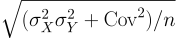correlation returns NULL on a degenerate (zero-variance) argument in every tier.

Collapsed aggregate moments

CollapsedAggMoment.cpp is the Rao-Blackwellised fast path for the recurring latent-variable relational shape: an aggregate over probabilistically-selected rows whose per-row selection events are coupled through one shared continuous latent. Conditional on that latent the row indicators are independent, so the aggregate’s moments collapse to a 1-D quadrature over the shared latent instead of an $n^k$ tuple enumeration or a degenerating importance sampler. It is exact up to the quadrature grid and works at provsql.rv_mc_samples = 0; complexity $O(n^2 + G\,K)$ (G grid points, K per-point cost). This is distinct from the foldDegenerateMixtures Bernoulli-arm collapse (see HybridEvaluator): that pass folds a certain ( $\pi \in \{0, 1\}$ ) Bernoulli selector to its surviving arm, whereas this one marginalises a fractional, shared continuous latent analytically.

Two entry points, both consulted by Expectation.cpp before the generic MC fallback and exposed as SQL:

aggCollapsedRawMoment (SQL agg_collapsed_moment (token, k) and the paired agg_collapsed_moments (token) that returns both {E[C], E[C²]} from a single circuit load) computes the raw moment $E[C^k]$ (k in {1, 2}) of a correlated COUNT / SUM by a Poisson-binomial 1-D quadrature over the shared latent, with the closed-form per-row CDF given it. It returns std::nullopt / SQL NULL when the circuit does not match the shared-latent shape, so the caller falls back to the exact $n^k$ enumeration. variance uses the paired form so a mean-plus-variance readout traverses the circuit once.
collapsedConditionalMoment computes the exact posterior raw moment $E[R^k \mid Y = C]$ of a latent R conditioned (through an equality event) on a discrete rv Y – parametrised by R – equalling a correlated COUNT C. The event must be a gate_cmp with = whose operands are a parametric discrete gate_rv over R and a gate_agg count; the count’s pmf $P(C = j)$ comes from the collapse, and the posterior is the second 1-D quadrature $E[R^k \mid C] = \int r^k f_R(r)\,L(r)\,dr / \int f_R(r)\,L(r)\,dr$ with likelihood $L(r) = \sum_j P(C = j)\,\mathrm{pmf}_Y(j; \theta(r))$ . A shape mismatch returns nullopt and the caller falls back to importance sampling.

HybridEvaluator

HybridEvaluator.cpp is the orchestrator. Given a circuit, it runs:

Universal peephole pass (runHybridSimplifier) that folds family-preserving combinations into a single leaf. The fold rules are registry-driven: try_sum_closure collects a PLUS gate’s wires as a·Z + b terms and consults the sum-closure registry (any linear combination of independent normals and constants into a single normal; a same-rate Exponential / Erlang chain into erlang(Σk, λ); same-rate Gammas into a Gamma); try_product_closure consults the product registry (independent lognormals fold in log space); try_transform_closure consults the transform registry (exp(Normal) → Lognormal, ln(Lognormal) → Normal – so a chain like exp(N_1 + N_2) collapses to one lognormal leaf). Scalar shifts, scalings, and negations of a single RV fold through Distribution::affine; a family whose affine image leaves the family declines the fold and the shape stays a gate_arith (shifting or negating an exponential, for instance, flips or displaces its support). Around the registry rules sit the structural canonicalisations: MINUS-to-PLUS (so subtraction shapes flow through the same PLUS pipeline), DIV-to-TIMES for division by a constant, shift-and-scale pushed through mixtures and categoricals, single-child arith roots, semiring-identity drops (gate_one in TIMES, gate_zero in PLUS…), and constant folding of deterministic subtrees – including POW / LN / EXP / MAX / MIN over constants, with domain-violating constants deliberately left unfolded so the sampler’s guard fires. The pass is invariant-preserving: every transformation produces a semantically equivalent circuit. Out of scope: combinations with no registered rule – the sum of two distinct uniforms (triangular, not uniform), differing-rate exponential sums, min / max of RVs (only their means have closed forms, see above); these shapes stay as gate_arith and the MC sampler handles them per-iteration.

Peephole is borrowed from compiler engineering (McKeeman, CACM 8(7), 1965): a small sliding window over consecutive instructions / gates, a fixed list of local pattern -> replacement rules, iterated to a fixed point. Each rule here looks at one gate_arith plus its immediate children, never further, matching the original scope. Contrast with RangeCheck (RangeCheck.cpp), which propagates a data-flow fact (the support interval) through the whole circuit, and with the island decomposer below, which uses a global union-find over base-RV footprints.
Island decomposition (runHybridDecomposer) that splits a multi-cmp query into independent islands (connected components on a union-find over base-RV footprints). A single-cmp island marginalises to a Bernoulli gate_input via AnalyticEvaluator. A multi-cmp island whose cmps share base RVs is enumerated via the joint table (the joint distribution of the shared base RVs is evaluated explicitly).
Monotone-shared-scalar fast path for the common shape of a single gate_rv shared across multiple monotone comparators (typical of range queries on a single column): the joint event reduces to an interval on the underlying scalar and one analytical CDF call per endpoint.

This fast path is analytical when the shared scalar is a bare gate_rv with a closed-form CDF, so the decomposer deliberately does not short-circuit on provsql.rv_mc_samples = 0: skipping it would leave the correlated cmps for AnalyticEvaluator to collapse one at a time, silently returning the product of the marginals for events that share a leaf (e.g. Pr(x ≥ 2000 ∧ x ≥ 1000) coming back as Pr(x ≥ 2000)·Pr(x ≥ 1000) rather than Pr(x ≥ 2000)). Only the genuinely MC-bound arms – a composite (non-gate_rv) shared scalar, an RV-vs-RV joint table, a non-analytic singleton – are gated on rv_mc_samples > 0; under 0 a correlated island with no closed form raises (a CircuitException surfaced as a clean error) rather than falling back to the independent product. This is what makes probability((A) | (B)) over two shared-leaf comparisons exact even with the MC fallback disabled.
Universal semiring-identity collapse after RangeCheck has decided every decidable cmp.

The simplifier is gated by provsql.simplify_on_load for the universal pass run at load time, and by the debug-only provsql.hybrid_evaluation (GUC_NO_SHOW_ALL) for the in-evaluator hybrid path. End users have no reason to flip hybrid_evaluation; it exists for developer A/B against the unfolded path and as a bisection knob.

Conditional Evaluation

expected, variance, moment, central_moment, quantile, support, rv_sample, and rv_histogram all accept an optional prov uuid DEFAULT gate_one() argument. When prov resolves to anything other than gate_one(), evaluation routes through the joint-circuit loader.

getJointCircuit (MMappedCircuit.cpp) builds a multi-rooted BFS over the union of the reachable gates from both input and prov so shared gate_rv leaves between the two are loaded into a single GenericCircuit and consequently couple correctly in the Monte Carlo sampler’s per-iteration caches. This is the shared-atom coupling invariant: a conditioning event prov is only meaningful relative to the random variables it references, and those must be the same leaves the moment’s evaluator sees.

The closed-form table for truncated (interval-conditioned) moments is a per-family capability, not a hard-coded list: a family implementing Distribution::truncatedRawMoment gets exact conditional moments (Normal via the Mills-ratio formula and integration by parts, Uniform trivially on the intersected interval, Exponential by memorylessness plus the lower incomplete gamma, Lognormal, Weibull, Pareto – the latter via tail self-similarity – and Beta via the incomplete-beta ratio). Families that decline (Erlang, Gamma) fall through to the MC path below. Extending the truncated surface to a new family means implementing truncatedRawMoment (and, for exact conditioned sampling, sampleTruncated) in that family’s file – no detection or dispatch site changes.

For shapes outside the closed-form table, the conditional moment is estimated by rejection sampling at provsql.rv_mc_samples; rv_sample emits a NOTICE (and rv_histogram / expected raise) when the acceptance rate drops below the requested n within the budget, so the caller can either widen the budget or loosen the conditioning.

matchTruncatedSingleRv (in RangeCheck.cpp) is the single-RV shape-detection helper used by the moment surface (try_truncated_closed_form in Expectation.cpp), the quantile evaluator, and the rejection-free sampler (try_truncated_closed_form_sample). It runs the four common gates – gate_rv root check, parse_distribution_spec, collectRvConstraints, and the empty-intersection / gate_zero event guards – so the supported-shape set stays in sync between moments, quantiles, and sampling.

matchClosedFormDistribution (same file) generalises the single-RV matcher to the four-arm variant std::variant<TruncatedSingleRv, DiracShape, CategoricalShape, BernoulliMixtureShape> consumed by rv_analytical_curves. The variant covers, in addition to the bare-RV case, as_random(c) Diracs (gate_value roots), categorical-form gate_mixture roots, and classic Bernoulli gate_mixture roots over any recursively-matched shape. A bare-RV root under conjugate observe-evidence resolves first through conjugatePosterior (the posterior is itself a bare distribution, returned as an untruncated single-RV shape – this is what makes rv_histogram and the curve renderers exact for recognised posteriors). Conditioning is honoured uniformly across all four arms: non-trivial events are routed through collectRvConstraints to extract a [lo, hi] interval on the root variable, then truncateShape is applied recursively – bare RVs intersect their bounds and renormalise via the truncated CDF; Diracs are kept iff the value falls inside the interval (otherwise the event is infeasible); categoricals drop outcomes outside the interval and renormalise surviving masses; Bernoulli mixtures recursively truncate their arms and reweight the Bernoulli by the ratio of arm masses ( $\pi' = \pi Z_L / (\pi Z_L + (1-\pi) Z_R)$ ), with the arm masses computed by shape_mass (a parallel recursive pass that integrates the unconditional CDF over the interval). An arm with zero post-truncation mass is eliminated and the mixture degenerates to the surviving arm.

eventIsProvablyInfeasible (also RangeCheck.cpp) is the conditional-moment dispatcher’s pre-MC short-circuit: gate_zero events are detected for every root type, and gate_rv roots additionally surface collectRvConstraints-empty intersections. The dispatcher in conditional_raw_moment / conditional_central_moment (Expectation.cpp) calls it after try_truncated_closed_form returns nullopt and raises a “conditioning event is infeasible” error directly when the predicate fires, avoiding a full rv_mc_samples MC round whose acceptance probability is exactly zero.

rv_sample and rv_histogram share MonteCarloSampler::try_truncated_closed_form_sample: a direct exact-sampling fast path that fires on a bare gate_rv with an interval-extractable event whenever the family implements Distribution::sampleTruncated (Uniform draws U(lo, hi) on the intersected truncation; Exponential one-sided uses memorylessness (X | X > c = c + Exp(λ)), two-sided uses inverse-CDF via std::log1p / std::expm1 for numerical accuracy near the support boundary; Normal uses the inverse-CDF transform; Lognormal, Weibull, and Pareto invert their exact quantiles). The fast path delivers exactly n samples with 100% acceptance even for tight tail events that would otherwise starve the rejection budget. Families without sampleTruncated (Erlang, Gamma, Beta, Inverse-Gamma, Inverse-Gaussian) and gate_arith composite roots fall through to MC rejection unchanged.

rv_analytical_curves (in RvAnalyticalCurves.cpp) exposes the closed-form PDF, CDF, and discrete stems as sampled data for ProvSQL Studio’s Distribution profile overlay. Returns NULL when the root sub-circuit is not a closed-form shape, so callers can dispatch it in parallel with rv_histogram without a structural pre-check. The payload has three optional fields:

pdf – evenly-spaced {x, p} samples of the continuous density. Absent when the shape has no continuous component (pure Dirac, pure categorical, or nested mixture of those).
cdf – same grid as pdf, cumulative probability. Always emitted (well-defined for any supported shape; a pure- discrete shape produces a staircase, a continuous shape a smooth curve, and a mixed shape a smooth curve with jumps at the stem positions).
stems – {x, p} point masses produced by Dirac roots, categorical roots, or Dirac / categorical arms inside a Bernoulli mixture. Bernoulli weights propagate down the path (a Dirac inside mixture(0.3, X, c) appears at (c, 0.7)).

The supported shape set is the union of matchClosedFormDistribution ‘s variant arms (see above): a bare gate_rv of any registered family – the plot window, density, and distribution come from Distribution::plotRange / pdf / cdf, so a new family gets curves for free; a family that declines pdf/cdf on the grid (NaN) returns NULL – plus as_random(c) Diracs, categorical mixtures, and Bernoulli mixtures over any recursively-matched shape, all four arms accepting a non-trivial conditioning event. gate_arith composites return NULL; the frontend renders histogram-only in those cases.

Before matching, rv_analytical_curves runs runHybridSimplifier so the curves see the same folded tree that simplified_circuit_subgraph exposes to Studio’s circuit view: c·Exp(λ) folded to Exp(λ/c), sums of independent normals folded to a single normal, exp(Normal) folded to its lognormal image, c + mixture(p, X, Y) pushed inside the mixture, etc. Without this pass a circuit that displays as a single Exp(0.5) node would still be seen by the matcher as a gate_arith composite of value(2) and gate_rv:Exp(1) and would silently fall back to histogram-only.

Truncation under a bare RV normalises the PDF by $Z = \text{CDF}(\text{hi}) - \text{CDF}(\text{lo})$ and rescales the CDF to [0, 1] over the conditioning interval. Under a Bernoulli mixture the truncated PDF is $f_{M|A}(x) = (\pi \cdot Z_L \cdot f_{L|A}(x) + (1-\pi) \cdot Z_R \cdot f_{R|A}(x)) / (\pi Z_L + (1-\pi) Z_R)$ with the per-arm normalisers $Z_L, Z_R$ computed by shape_mass. Under a categorical the conditional masses are $p_i \cdot \mathbb{1}\{v_i \in A\} / \sum_j p_j \cdot \mathbb{1}\{v_j \in A\}$ . A Dirac is invariant under any feasible event.

The load-time pass runConstantFold (in HybridEvaluator.cpp, invoked from CircuitFromMMap::applyLoadTimeSimplification alongside runRangeCheck and foldSemiringIdentities) folds deterministic gate_arith subtrees to gate_value at load time. This lifts the common parser shape arith(NEG, value:c) (produced when SQL parses -c::random_variable as -(c::random_variable)) into a clean value:-c, so asRvVsConstCmp and friends recognise the comparator’s constant side without callers having to parenthesise. The pass runs only the constant-fold rule from the hybrid simplifier, never the family closures or identity drops, because the result is always a gate_value that carries no random identity, so no shared-RV coupling is decoupled by the rewrite. The family closures stay behind the separate provsql.hybrid_evaluation GUC, which gates runHybridSimplifier inside the probability and view paths where the simplifier owns the rewritten subtree.

Immediately before runConstantFold in the same load-time sequence, foldDegenerateMixtures collapses a classic Bernoulli mixture(p, X, Y) whose selector p is certainly true or false to the surviving arm: X when $\Pr(p) = 1$ , Y when $\Pr(p) = 0$ . The weight is read only where it is known without a probability computation – a resolved gate_one / gate_zero selector, or a bare gate_input whose pinned probability is exactly 1 or 0 (the default 1 of a non-probabilistic tuple included). The collapse rewrites the mixture as a single-wire gate_arith PLUS passthrough to the survivor (liftConditionedToTarget), which references rather than copies it, so a shared survivor keeps its single gate identity and single Monte-Carlo draw; foldSemiringIdentities then unwraps the passthrough. Ordering it before the constant fold is what lets a provenance-weighted count of certain tuples (the denominator of the avg rewrite, see Aggregate Dispatch) reduce to a gate_value. The fold is exact and correlation-safe precisely at $\pi \in \{0, 1\}$ : a deterministic selector shared across several mixtures couples none of them, whereas a fractional selector genuinely does, so the pass admits only the two endpoints and leaves every fractional Bernoulli for the Monte-Carlo sampler. A compound Boolean selector – whose $\Pr(p)$ would need a (possibly #P-hard) evaluation and depends on mutable input probabilities – is left intact for the probability-aware evaluators.

Information Theory

InformationTheory.cpp implements the entropy / Kullback-Leibler / mutual-information readouts, all in nats, over scalar RV sub-circuits. The exact paths resolve a gate to a closed density view – a bare gate_rv (its family pdf over the integration range), a gate_value / categorical mixture (a finite pmf), or a Bernoulli mixture tree over independent such arms (e.g. the gmm cascade) – and evaluate the defining integral or sum directly. Entropy of a discrete view is Shannon entropy (a point mass has entropy 0); of a continuous view, differential entropy (quadrature of $-f \ln f$ over the family’s integration range). The three C entry points are computeEntropy, computeKL, computeMutualInformation, bound to the SQL entropy (x [, prov]), kl (p, q), and mutual_information (x, y).

Entropy. Shapes with no closed density (arithmetic composites) and the conditional form (prov other than gate_one()) fall back to a Monte Carlo histogram plug-in estimate at the provsql.rv_mc_samples budget.
KL divergence. Exact only: the defining sum for two discrete views (outcomes matched by value) and the defining integral (quadrature over P’s integration window) for two continuous ones, including independent-arm mixture trees. Returns Infinity when P is not absolutely continuous with respect to Q (mismatched kinds, an atom or region of P outside Q’s support). KL has no density-free estimator, so an arithmetic composite or conditioned argument raises rather than falling back to Monte Carlo.
Mutual information. Exactly 0 for structurally independent roots (disjoint stochastic-leaf footprints, the same FootprintCache test the moment evaluators use); H(X) for a discrete variable paired with itself and Infinity for a continuous one (I(X; X) diverges); a genuinely correlated pair (shared leaves) is the 2-D histogram plug-in over coupled joint draws – both roots evaluated against the same per-iteration cache so shared leaves keep their joint law – at the provsql.rv_mc_samples budget.

Aggregate Dispatch

The sum, avg, product, max, and min aggregates over random_variable all share sum_rv_sfunc as their state-transition function (a uuid[] accumulator) and an INITCOND = '{}' so the FFUNC runs even on an empty group.

The row-absence identity is baked into each per-row contribution upstream, by the planner hook: make_rv_aggregate_expression wraps the per-row argument in rv_aggregate_semimod – a mixture (prov_i, X_i, as_random(identity)) – with the identity dispatched per aggregate: 0 for sum (the two-argument form), and, through the three-argument identity-parameterised form, 1 for product, -Infinity for max, +Infinity for min – a row absent in a world must not perturb the fold, so it contributes the fold’s identity. avg is rewritten at the same site into the “AVG = SUM / COUNT” identity, rv_sum_or_null(rv_aggregate_semimod(prov, x)) / sum(rv_aggregate_indicator(prov)): the numerator is the usual provenance-weighted sum (rv_sum_or_null differs from sum only in returning NULL on an empty group so the division propagates standard AVG semantics), and the denominator sums per-row mixture(prov_i, 1, 0) indicators – the count of included rows as a random variable.

That denominator is a genuine random variable only when some row is uncertainly present. When every contributing tuple is certain – the default for a provenance-tracked but non-probabilistic table, where each input gate carries the default probability 1 – the count is deterministic, and expected(avg(x)) is simply E[SUM] / n. The load-time foldDegenerateMixtures pass (see HybridEvaluator) turns this into an analytic result: a Bernoulli mixture whose selector is certainly true ( $\pi = 1$ ) or false ( $\pi = 0$ ) is collapsed to the surviving arm, so each denominator mixture(prov_i, 1, 0) becomes the constant 1 and constant folding reduces the whole sum to the gate_value $n$ that the analytic DIV-by-constant arm divides by (each numerator mixture(prov_i, X_i, 0) likewise unwraps to X_i, leaving a plain sum of the row RVs). A fractional presence probability genuinely couples the numerator’s random sum to the random count, so its mixtures are left intact and the ratio is estimated by Monte Carlo – the fold admits only the exact $\pi \in \{0, 1\}$ cases, where a deterministic selector carries no coupling to lose.

With the identities pre-baked, the FFUNCs are plain folds with no gate inspection: a single gate_arith root (PLUS / TIMES / MAX / MIN, the extremum pair through the shared extremum_rv_ffunc) over the accumulated UUIDs, a singleton group collapsing to its single child, and per-aggregate empty-group identities (as_random(0) for sum, as_random(1) for product, as_random(∓∞) for the extrema, SQL NULL for avg). On an untracked call (no provenance to weight by) the direct aggregates still work: every row is unconditionally present and the raw per-row RVs are folded as-is.

The dispatch is keyed on aggtype (the aggregate’s result type OID) rather than aggfnoid so the same routing works for any future RV-returning aggregate.

An earlier design considered an M-polymorphic gate_agg that would carry the full semimodule lift directly. We rejected it because the mixture-of-mixtures shape composes through every existing gate_arith / gate_mixture rule, while a new M-polymorphic gate would have required a parallel evaluation path in every analytical evaluator. The semimodule-of-mixtures shape reuses what’s there.

Statistic aggregates

The SQL-standard statistic aggregates (covar_pop / covar_samp / corr two-argument, stddev_pop / stddev_samp one-argument, and the ordered-set percentile_cont) use a different wrap: instead of baking a fold identity into each row’s mixture, they carry the row’s presence indicator explicitly. The public aggregates append the certain indicator as_random(1) per row; a provenance-tracked query is rewritten by make_rv_aggregate_expression to the internal rv_*_impl aggregates, whose extra leading argument is rv_aggregate_indicator(prov) (the mixture(prov, 1, 0) indicator avg already uses), so absent rows drop out of every sum, the count, and the percentile member set.

The moment statistics are then pure circuit arithmetic over indicator-weighted power sums – rv_stat_sum_tokens mints $N = \sum \mathbf{1}_i$ , $S_X$ , $S_{XX}$ (and $S_Y, S_{XY}, S_{YY}$ for the two-argument forms) as gate_arith PLUS-of-TIMES trees, sharing each row’s indicator gate between $N$ and every product it weighs so the Monte Carlo per-iteration cache keeps presence coupled across the sums (and a repeated wire [ind, x, x] reuses the same draw of x, giving $x^2$ ). No new opcode is needed: e.g. covar_pop is MINUS(DIV(SXY, N), TIMES(DIV(SX, N), DIV(SY, N))), and the stddevs clamp the variance with MAX(v, 0) before POW(·, 0.5) so floating-point error can never trip the pow domain guard. Undefined worlds ( $N = 0$ ; $N = 1$ for the sample forms; zero variance for corr) evaluate to NaN, the established convention the moment estimators skip.

percentile_cont is the one statistic arithmetic cannot express: it mints the appended PROVSQL_ARITH_PERCENTILE (= 10) gate_arith whose wires are the interleaved [ind_1, x_1, ..., ind_n, x_n] pairs and whose fraction is text-encoded in extra (and participates in the token UUID, so two fractions over the same group are distinct gates). The Monte Carlo sampler arm collects the values whose indicator draws 1, sorts, and linearly interpolates; RangeCheck propagates the hull of the value wires’ supports; the moment evaluators route it straight to the sampler (no closed form). Because the planner rewrite replaces the ordered-set Aggref with the normal three-argument rv_percentile_impl before planning, the executor never sorts random_variable rows – the sort order is irrelevant to the gate – which is also why the untracked public form is unusable: its input sort funnels into random_variable_btree_cmp and raises. The fraction travels as the leading impl argument into a composite transition state (rv_percentile_state), since a normal aggregate’s final function sees only the state.

Studio Rendering

ProvSQL Studio’s circuit canvas is class-based: every node carries a node--<type> CSS class derived from the gate kind, and the stylesheet at studio/provsql_studio/static/app.css gives each class its colour, glyph, and inline-text layout. The continuous gate types map to:

one entry per type in the server-side JSON serialiser at studio/provsql_studio/circuit.py (the label and children fields, plus the distribution-blob parsing for the per-leaf inline glyph);
one branch in the client renderer at studio/provsql_studio/static/circuit.js to pick the node--rv / node--arith / node--mixture / node--case class and to emit the correct edge labels (p / x / y for mixtures; the provsql_arith_op glyph for arith, with pow(x, 0.5) rendered as √; guard / value / default for gate_case, whose node glyph is ⇢);
a Circuit-mode fetch that consumes the simplified_circuit_subgraph function (SimplifiedSubgraph.cpp), which runs the universal peephole pass on a sub-BFS and returns the result as a single jsonb value, with the provsql.simplify_on_load Config-panel toggle switching between the raw and folded views.

The RV-family rendering is registry-driven end to end: Studio reads rv_families for each family’s display label and parameter symbols, and fetches its density preview as a server-computed grid from rv_analytical_curves – so a newly registered family renders correctly with no Studio change.

The eval-strip Distribution profile, Sample, Moment, and Support entries call rv_histogram, rv_sample, rv_moment and rv_support directly. The Condition on row-prov auto-preset is a client-side feature: clicking a result cell stamps the row’s provenance UUID into the input and toggles the Conditioned by badge active. Manual edits stick within a row; row navigation resets the input to the new row’s prov.

Latent variables and posterior inference

A distribution parameter may be a scalar provenance token instead of a literal double, making the leaf a compound (hierarchical) distribution; conditioning such a leaf on observed data is likelihood-weighting posterior inference. Two mechanisms implement this.

Parameter wires on gate_rv. A gate_rv gained the ability to carry wires (it never did before, so no mmap format bump is needed). A parameter slot in the extra text is either a literal or a wire reference $i (0-based index into the gate’s wire vector), e.g. "normal:$0,1.0". DistributionSpec (the resolved {family, double, double} POD every analytic call site consumes) is unchanged; a parallel template parser (parse_distribution_template in src/RandomVariable.cpp, returning DistributionTemplate with per-slot DistributionParam) keeps the literal-or-wire distinction, and parse_distribution_spec is now that template parse followed by an all-literal check – so it declines a parametric leaf and every analytic path (Expectation.cpp, AnalyticEvaluator.cpp) falls through to Monte Carlo unchanged. The sampler’s gate_rv arm (src/MonteCarloSampler.cpp) resolves wired parameters per iteration through evalScalar (so a shared latent lands in scalar_cache_ and couples the leaves) and builds the family instance for that draw; integrationRange() is the family-agnostic domain guard for a drawn-out-of-support parameter. The FootprintCache unions a latent leaf’s parameter-wire footprints into its own, so two leaves sharing a latent are flagged dependent and the independence shortcuts defeat correctly. The DistributionFamily factory and the Distribution interface are untouched – only the parameters’ source (sampled wire vs literal) changes.

The gate_observe evidence gate and importance sampling. gate_observe (append-only enum addition; one wire → the observed gate_rv leaf, the datum in extra) is an evidence node: it composes into an evidence circuit by gate_times exactly like a Boolean conditioning event, but contributes a continuous density factor. Sampler::evalWeight walks the evidence circuit to a weight rather than a bool or scalar: a gate_observe returns its leaf’s pdf at the datum (resolving the leaf’s latent parameters through evalScalar, so the weight and the value couple), a gate_times multiplies its children’s weights, and any other subtree falls to evalBool for a 0/1 weight – so a purely Boolean evidence tree reproduces the rejection conditioning. importanceSampleConditional draws latents from the prior, weights each by evalWeight(evidence), and returns a WeightedPosterior of (value, weight) particles plus the marginal likelihood P(data) (mean weight) and the effective sample size (Σw)² / Σw². The moment / quantile / sample dispatchers route to it whenever circuitHasObserve finds a gate_observe in the evidence and the exact conjugate recogniser below has declined, computing weighted posterior statistics (rv_sample resamples the particles, SIR). The whole readout goes through getJointCircuit so a latent shared between the root and the evidence is a single gate_t.

Exact conjugate posteriors. ConjugatePosterior.cpp is the closed-form fast path over the same evidence surface: when the target is a bare all-literal gate_rv (the prior), the evidence flattens through the gate_times spine into gate_observe atoms only (gate_one factors are skipped; any other factor declines), and every observed leaf’s DistributionTemplate has exactly one wired slot whose wire is the target gate itself, the posterior is folded one observation at a time through the conjugate-update registry (registerConjugateRule in distributions/Distribution.h, keyed on (likelihood family, wired parameter position, running posterior family) – the same self-registering name-token pattern as the comparator / closure / transform registries, one rule per likelihood family file). The result is a first-class DistributionSpec of the prior’s family, so ONE recognition upgrades every readout at once:

conditional_raw_moment / conditional_central_moment (Expectation.cpp) return the family’s closed-form moments – the attempt slots between collapsedConditionalMoment and the circuitHasObserve importance-sampling fallback, preserving the invisible-fallback guarantee (any nullopt leaves the ladder unchanged);
compute_quantile inverts the posterior CDF exactly;
rv_sample draws i.i.d. from the posterior distribution (no weighted-particle resampling), seeded through the shared seedRng;
matchClosedFormDistribution (RangeCheck.cpp) returns the posterior as an untruncated TruncatedSingleRv shape, making rv_histogram and rv_analytical_curves exact;
computeEntropy (InformationTheory.cpp) integrates the posterior pdf exactly;
evidence returns exp(Σ log m(dᵢ | ...)), the exact marginal likelihood from each rule’s log_predictive (the sequential chain-rule factorisation, accumulated in log space); a rule without a predictive declines the whole evidence recognition.

Everything works at provsql.rv_mc_samples = 0. Each rule’s update guards its own domain (an out-of-support datum, an invalid literal slot, a non-integer count outside the family pmf’s 1e-9 rounding tolerance) and declines rather than raises – the zero-weight / ESS diagnostics of importance sampling remain the UX for contradictory evidence. The fold canonicalises an erlang or exponential prior into the gamma carrier (identical distributions; the SQL gamma constructor stores an integer-shape prior as an erlang leaf). Because conjugacy is checked per observation against the running posterior family, mixed likelihoods sharing one conjugate prior compose (Poisson counts and Exponential gaps over one Gamma-prior rate). Correctness is by construction the importance- sampling estimand: the IS weight is exactly ∏ f(dᵢ | θ) (evalWeight) and the conjugate posterior is the prior times that product renormalised, so recognition changes the method, never the semantics. The MVP rule table covers Normal-Normal (mean slot), Normal-LogNormal (log-location), Gamma-Exponential / -Poisson / -Gamma / -Erlang / -Pareto (rate and tail-shape slots), Beta-Binomial / -Geometric / -NegativeBinomial (success-probability slots, in each family’s own support convention), and Pareto-Uniform (upper bound, zero lower bound only – 1/(θ−a₀) is Pareto-shaped in θ only for a₀ = 0). Deliberately absent, because the exact posterior leaves the registered families (so it cannot ride the DistributionSpec carrier): a prior on a Normal’s σ slot (conjugacy is on the precision, not σ), a Beta likelihood with a latent shape (the 1/B(α, β) normaliser puts Gamma-function factors in the posterior kernel), Weibull’s scale slot, and multi-latent / hierarchical posteriors. All decline to importance sampling. The regression file is continuous_conjugate.sql (exact pairs at rv_mc_samples = 0, plus decline coverage validated against IS).

The discrete families (poisson, binomial, geometric, negative_binomial) are ordinary self-registering Distribution subclasses (isDiscrete() == true) that happen to be integer-valued: sample() draws from the matching std::…_distribution, pdf() is the pmf (the observe likelihood weight), and integrationRange() doubles as the parameter-domain gate (λ > 0; 0 ≤ p ≤ 1; 0 < p ≤ 1). They are only ever instantiated for a latent leaf – poisson(random_variable), binomial(integer, random_variable), geometric(random_variable), negative_binomial(r, random_variable) – because the literal constructors still enumerate an exact categorical; and a parametric leaf is declined by parse_distribution_spec, so no continuous-analytic path ever integrates their pmf as a density. They reuse the parametric- leaf mechanism wholesale, which is why the discrete conjugate posteriors (Gamma-Poisson, Beta-Binomial) fall out with no evaluator change. hypergeometric stays literal-only: its three parameters do not fit the two-parameter Distribution ABI, so there is no parametric-leaf form – the constructor always enumerates its exact categorical.

The equality-form surface. The user writes the natural conditional-equality X | (Y = c) (single) or given(Y = c) folded by and_agg (a table); observe is the internal primitive. The bridge is evidence_as_observation (SQL): when a conditioning event is a gate_cmp with the = operator, one side a bare gate_rv leaf and the other a constant, it is rewritten to a gate_observe at construction time – so the stored evidence never reaches the load-time measure-zero fold. random_variable_cond (the | operator) and given both apply it; given(boolean) (the renamed given_predicate placeholder) is planner-rewritten from both the | (predicate) operator and the given(predicate) function call.

This is where the Distribution::isDiscrete() flag earns its keep. A point event Y = c is measure-zero for a continuous leaf (folded to gate_zero by RangeCheck’s continuous EQ/NE shortcut and Dirac sum-product) but positive-mass for a discrete one; isDiscrete() (an authoritative per-family flag, propagated through transforms by hasOnlyContinuousSupport / collectDiracMassMap) keeps the discrete equality from folding, so a discrete selection (probability(poisson = 5)) stays exact while a discrete/continuous conditioning Y = c is routed to likelihood weighting through the observe rewrite.

The rest of the SQL surface is evidence / shapley_observe, the token-accepting constructor overloads, and the provsql.ess_warn_fraction GUC. shapley_observe is connecting code: it enumerates the observation subsets, calls rv_moment for each coalition’s posterior value, and combines them into the Shapley attribution – exact, so capped at 12 observations. Sequential Monte Carlo (for the many-observations regime where the ESS collapses) and MCMC are deferred: the sampler is stateless (resetIteration() wipes state each draw) and has no joint-density-at-an-assignment evaluation mode, which MCMC’s acceptance ratio needs.