Case Study: The City Air-Quality Sensor Network

This case study demonstrates ProvSQL’s continuous-distribution surface (see Continuous Distributions) end-to-end through ProvSQL Studio (see ProvSQL Studio). It is the first case study driven primarily by Studio rather than psql: random variables benefit far more from interactive visualisation – PDFs, CDFs, mixture DAG layouts, conditional histograms, simplifier before-vs-after – than from text-mode output, and the workflow below makes the rewriter, the simplifier, the analytic and Monte-Carlo paths, and conditional inference all visible in the canvas.

The Scenario

A municipal observatory operates a small air-quality sensor network. Sensors of three different vendors report a concentration (fine particulate matter, i.e. airborne particles with aerodynamic diameter at most 2.5 μm, expressed in micrograms per cubic metre) on a fixed schedule. The sensors differ in calibration and noise characteristics:

• high-end units report Normal(μ, σ) with small σ;

• low-cost units report Uniform[μ−δ, μ+δ] over a small window;

• a drift-prone unit reports Exponential(λ) while its internal hardware self-tests cycle;

• a multi-pass aggregating unit reports Erlang(k, λ) over the pass count.

A reference station with a calibrated lab-grade instrument contributes deterministic readings.

Regulatory categories partition the value axis: Good below 12, Moderate between 12.1 and 35, Unhealthy above 35.1 (loosely following the US EPA AQI breakpoints for PM2.5 in their pre-2024 form, simplified to three tiers). Each station has a Bernoulli probability of being in calibration on a given day. A separate batch table of historical readings carries the same shape so cross-batch queries via UNION ALL are meaningful.

Your tasks:

• inspect the per-row distributions and the rewriter’s effect on threshold queries;

• compute the probability that each station’s reading exceeds an Unhealthy threshold, exercising the planner-hook rewrite for WHERE reading > 35;

• model calibration uncertainty as a Bernoulli mixture and inspect the resulting gate_mixture shape;

• aggregate per-district readings and watch the simplifier fold the mixture cascade;

• run conditional inference (E[reading | reading > 35]) and see the closed-form truncated-distribution mean against the unconditional one;

• filter on the expected value of an aggregated random variable, combine today’s and yesterday’s batches with UNION ALL, and compare probability methods ('independent' vs 'monte-carlo' vs 'tree-decomposition') side by side.

Setup

This case study assumes a working ProvSQL installation (see Getting ProvSQL) and a running ProvSQL Studio session pointed at it (see ProvSQL Studio). Download setup.sql and load it into a fresh PostgreSQL database:

createdb air_quality_demo
psql -d air_quality_demo -f setup.sql

The script creates the schema below and seeds the random-variable readings via the constructors documented in Continuous Distributions. It is five tables:

• stations(id, name, district) – four monitoring stations across two districts, provenance-tracked.

• readings(station_id, ts, pm25 random_variable) – one pm25 reading per station per timestamp; the random_variable carries the per-station noise model (normal, uniform, exponential, erlang, or a deterministic lifted from the reference station).

• calibration_status(station_id, p) – Bernoulli probability that each station is in calibration on the day of interest.

• categories(name, lo, hi) – three regulatory categories (Good / Moderate / Unhealthy) keyed by their interval bounds.

• historical_readings(...) – same shape as readings, populated from yesterday’s batch.

Connect Studio to the fixture:

provsql-studio --dsn postgresql:///air_quality_demo

and open http://127.0.0.1:8000/ in a browser. The schema panel lists the fixture’s six relations: the four provenance-tracked tables (stations, calibration_status, readings, historical_readings) carry the purple prov pill, categories is plain, and station_mapping is tagged mapping. The pm25 column on readings and historical_readings is flagged with a terracotta rv pill: a heads-up that comparison and arithmetic operators on this column are intercepted by the planner hook and lifted into provenance gates, so a query like pm25 > 35 produces a circuit rather than a Boolean.

The schema panel opened from the top nav. The four provenance-tracked tables carry the purple prov pill; readings and historical_readings list pm25 with a terracotta rv pill marking it as a random_variable column.

Step 1: Inspect a Noisy Reading

In the Studio query box:

SELECT id, ts, pm25
FROM readings
WHERE station_id = 's1'
ORDER BY ts

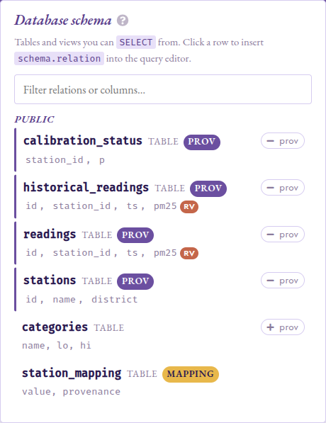
The result table renders pm25 as a clickable random_variable cell carrying the underlying gate UUID. Click into a row’s pm25: Studio switches to Circuit mode and renders the gate_rv leaf with the distribution-kind initial in the circle (N for a Normal, U for Uniform, Exp for Exponential, Erl for Erlang). Pick Distribution profile from the Distribution group of the eval strip and click Run: the panel returns and headline stats and an inline histogram with a PDF/CDF toggle.

The histogram is backed server-side by rv_histogram; pinning provsql.monte_carlo_seed in the Config panel (under Provenance) makes the shape reproducible across re-runs.

The gate_rv leaf for pm25 on row 1 is a N(28, 2) circle; the eval-strip Distribution profile panel shows the , , support, and an inline histogram. When the gate has a closed-form family (here a bare Normal), Studio overlays the analytical PDF on top of the bars; the curve rides the histogram envelope so any mismatch between the sampled histogram and the closed-form shape is immediately visible.

Step 2: A First Probabilistic Threshold

The Unhealthy category begins at 35.1. Find the rows whose reading might cross it:

SELECT id, station_id, ts
FROM readings
WHERE pm25 > 35

Because pm25 is a random variable, the comparison is not a yes/no test: it stands for the event “this reading exceeds 35”, and ProvSQL attaches that event to each row’s provenance.

Click into a result row’s auto-added provsql cell. Circuit mode shows the Boolean wrapper (a gate_times over the row’s input token and the gate_cmp); the cmp’s child link reaches into the gate_rv from Step 1.

The eval strip’s probability_evaluate entry exposes the five compiled methods (see Probabilities). Pick monte-carlo and set n = 10000; the panel returns the probability with a Hoeffding confidence band. Pin provsql.monte_carlo_seed = 42 in the Config panel and re-run: the result is now identical across runs. Toggle the seed back to -1 and re-run to see the band shift between runs.

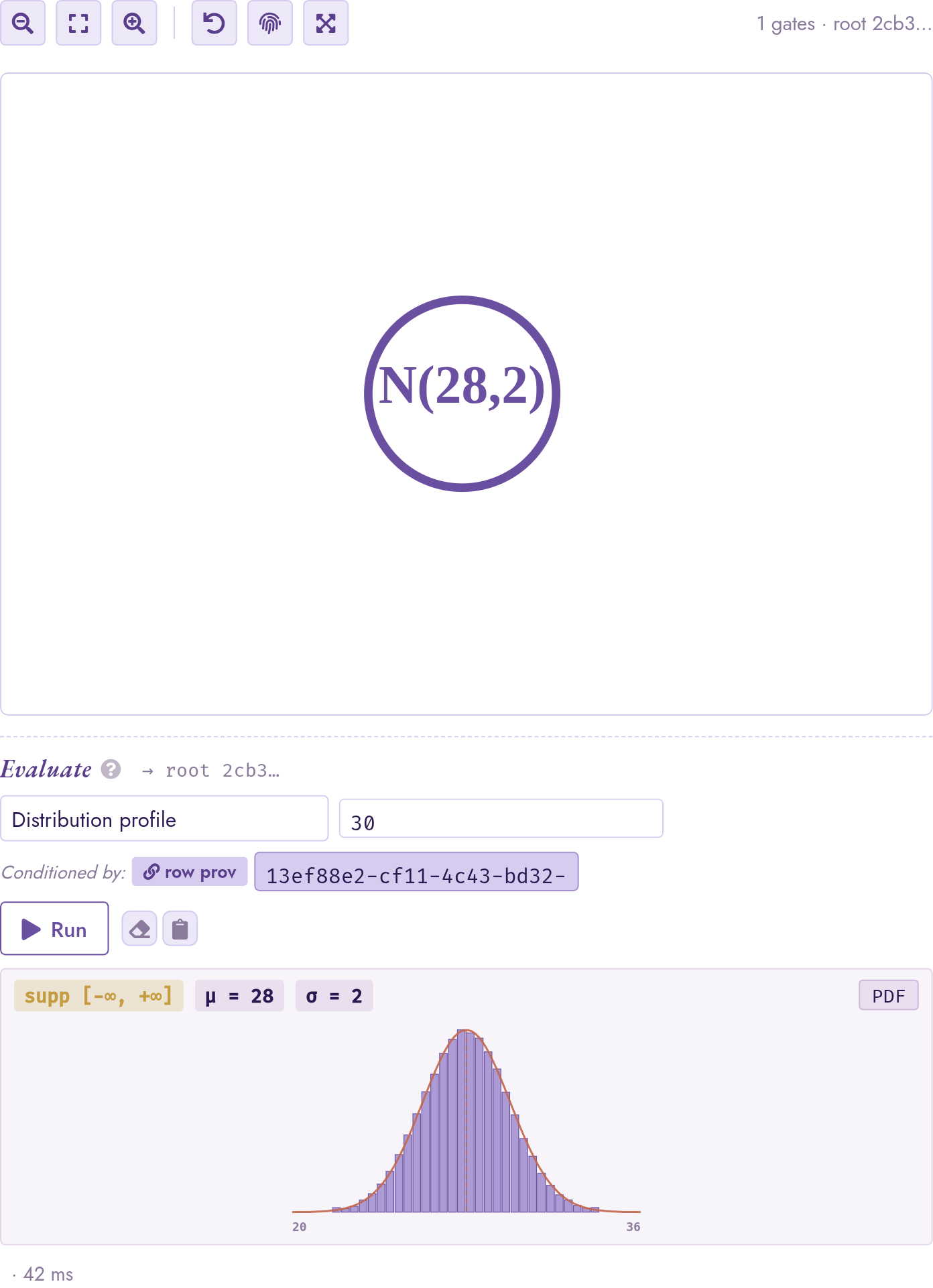
The provenance of one row from WHERE pm25 > 35: a gate_times (⊗) wraps the row’s input token ι and a gate_cmp > whose children are the N(28, 2) leaf and the constant 35. The eval strip below switches to probability_evaluate and exposes the method picker.

Step 3: The Simplifier in Action

The planner hook emits the comparator as a raw gate_cmp regardless of what its operands look like. A simplifier pass then folds comparators whose answer can be decided from the operand support alone — for example, U(10, 22) > 35 is universally false because the uniform’s upper bound is below the threshold. The fold is controlled by provsql.simplify_on_load (default on), which the Config panel exposes under Provenance.

Click into row 2’s auto-added provsql cell from the Step 2 result (station s2, pm25 ~ U(10, 22)). With provsql.simplify_on_load on, the canvas shows a single 𝟘 (zero) gate: the simplifier resolved the comparator to a constant-false leaf and dropped the whole subtree. Toggle the GUC off in the Config panel and click the cell again: the canvas now shows the raw construction shape, a gate_times (⊗) over the row’s input token ι and a gate_cmp (>) whose children are the U(10, 22) leaf and the constant 35. Both views are semantically identical; the simplified view is what the semiring evaluators and the Monte-Carlo sampler actually consume.

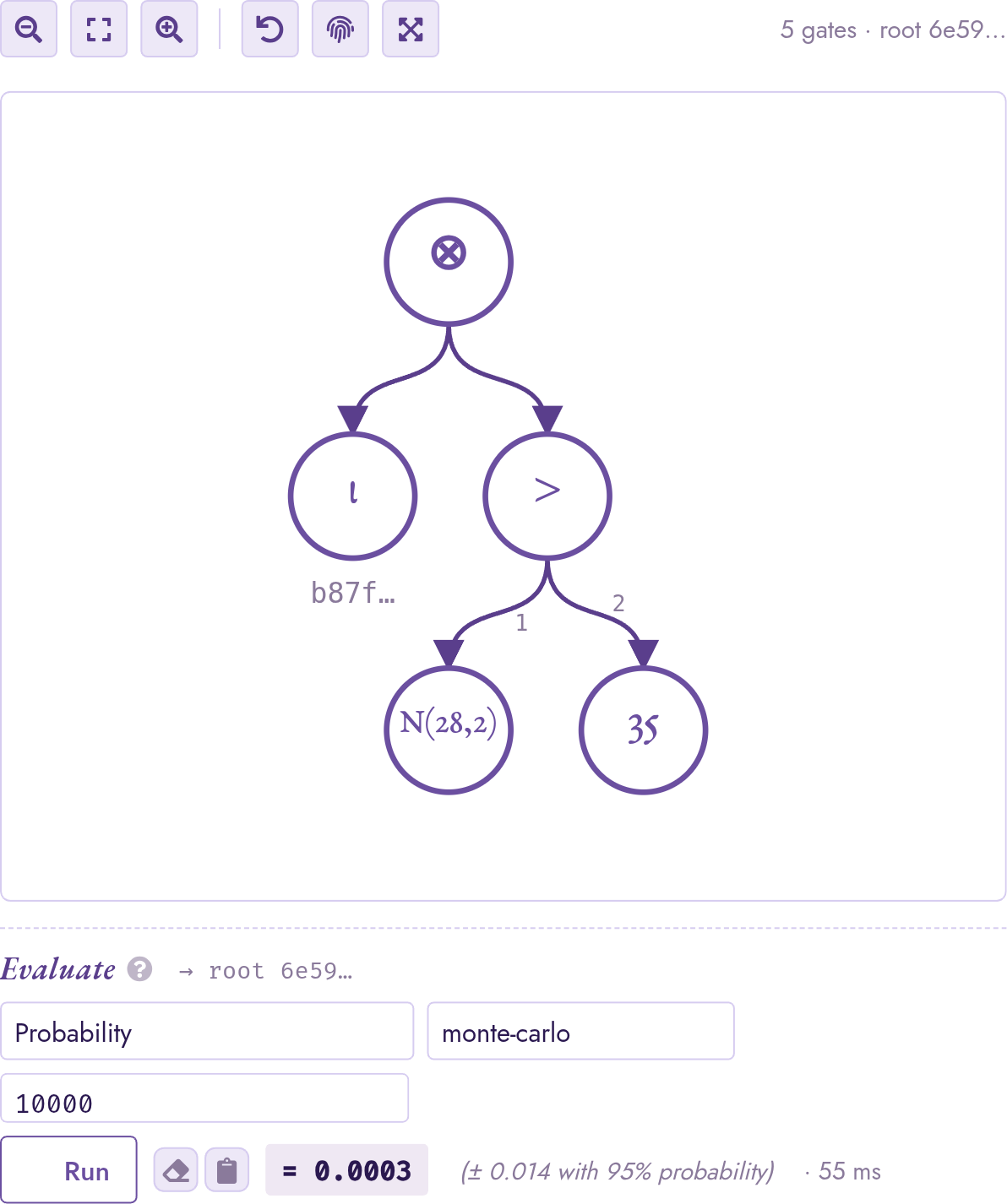
Row 2’s provenance for pm25 > 35 with provsql.simplify_on_load toggled off (left) vs on (right). The simplifier recognised that the upper bound of U(10, 22) is below the threshold, so the comparator is universally false and the whole subtree collapses to the additive identity 𝟘.

Step 4: Calibration via Mixtures

Each station has a probability of being mis-calibrated; a mis-calibrated unit over-reports by 20% (the reading it records is 1.2 times the true value). The corrected estimate of the true reading is therefore pm25 with probability p (the station is in spec) and pm25 / 1.2 with probability 1 - p (the report needs to be scaled back). Express this as a Bernoulli mixture:

SELECT r.id, r.station_id,
       provsql.mixture(cs.p, r.pm25, r.pm25 / 1.2) AS pm25_calibrated
FROM readings r JOIN calibration_status cs USING (station_id)
WHERE r.station_id = 's1'

Click into a result row’s pm25_calibrated cell. Circuit mode renders the gate_mixture as a Mix node with three labelled outgoing edges (p / x / y) matching the SQL constructor’s argument order: p points to the Bernoulli mixing probability, x to the in-spec arm, and y to the correction arm.

The same node-inspector panel exposes Distribution profile on the mixture root. Because station s1 is in spec 95% of the time, the histogram is dominated by the N(28, 2) arm and the out-of-spec N(23.33, 1.667) contributes only a small left shoulder rather than a visually distinct second mode; the panel headline reflects this with a mixture mean slightly below 28. To see clear bimodality, re-run the query with a larger calibration error — e.g. replace r.pm25 / 1.2 with r.pm25 / 2.0 so the out-of-spec arm folds to N(14, 1), well separated from the in-spec N(28, 2); the two peaks then show up distinctly on the histogram even at the 95%/5% weighting.

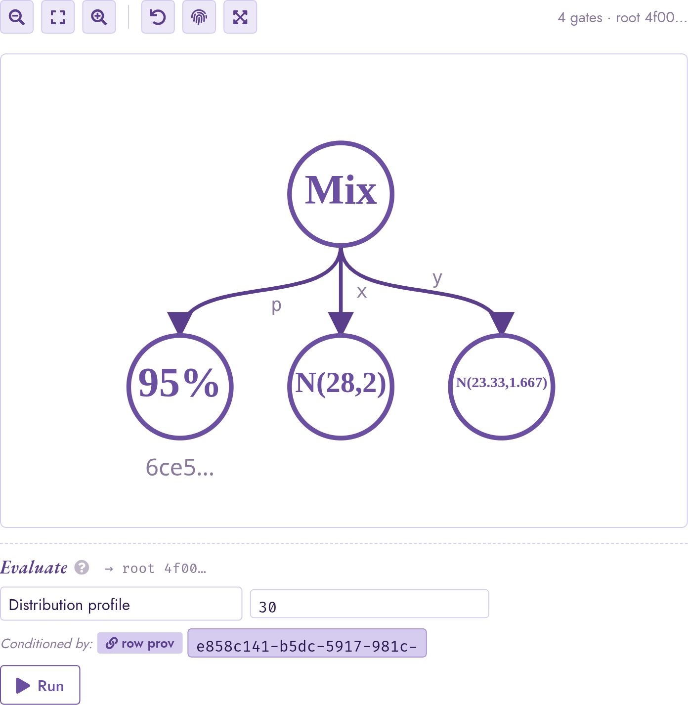
The gate_mixture for the calibrated reading. The 95% child is the Bernoulli probability that station s1 is in spec; the x arm is the raw reading N(28, 2); the y arm is the back-scaled estimate pm25 / 1.2, which the simplifier folded through the Normal affine-shift rule into a single gate_rv N(23.33, 1.667). Circle labels show four significant figures; the inspector pinned to either child surfaces the full-precision parameters.

Step 5: Aggregation Over Random Variables

Compute average per district:

SELECT s.district,
       avg(r.pm25)  AS avg_pm25,
       sum(r.pm25)  AS total_pm25
FROM readings r JOIN stations s ON s.id = r.station_id
GROUP BY s.district

Click into a row’s avg_pm25 cell. Circuit mode shows the avg lowering: a gate_arith(DIV, num, denom) over two gate_arith(PLUS, …) subtrees, each child a per-row gate_mixture produced by rv_aggregate_semimod. The right child of the outer division is the count of included rows under their per-row provenance: rows whose provenance is false contribute the additive identity to both numerator and denominator. Run Distribution profile on the root: the panel shows the per-district average as a tight distribution centred at the inclusion-weighted mean.

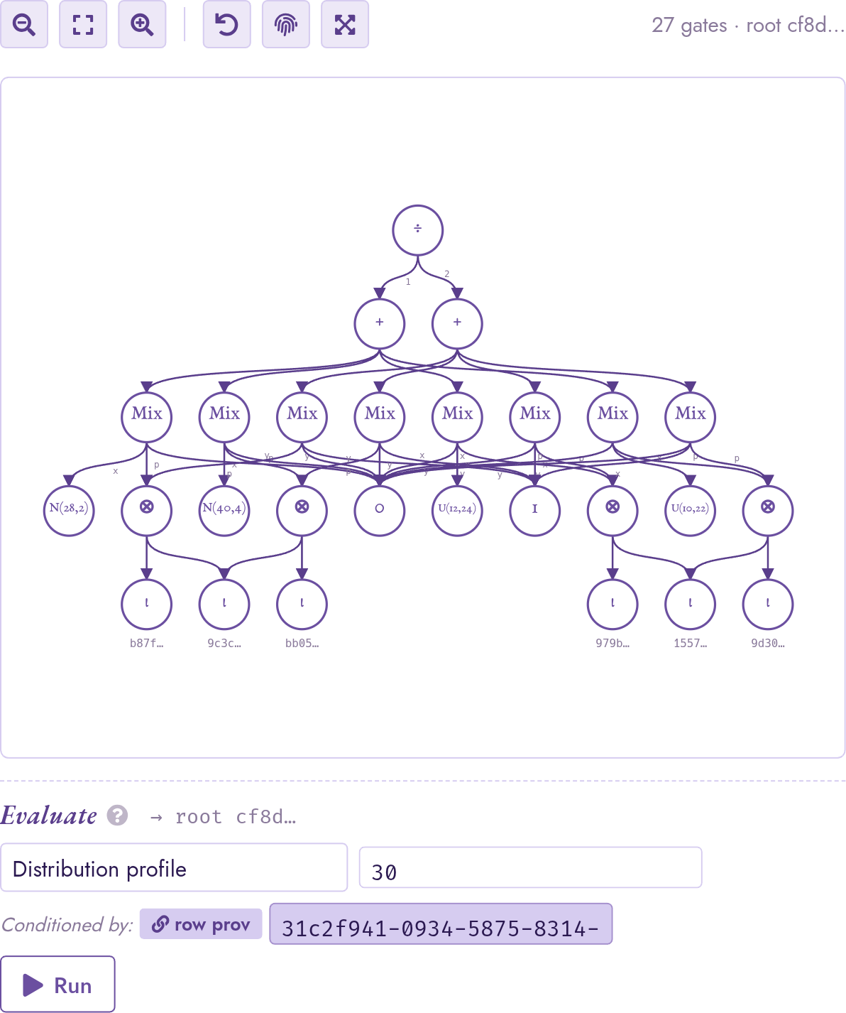
The avg(pm25) cell for the centre district lowers to gate_arith(DIV, gate_arith(PLUS, mixtures), gate_arith(PLUS, one-mixtures)). The eight mixtures correspond to the four stations × two timestamps that fall in the district; the gate_rv leaves at the bottom are the per-reading distributions; the ι leaves anchor each row’s provenance.

Step 6: Conditional Inference

Re-open the filtered query from Step 2:

SELECT id, station_id, ts, pm25
FROM readings
WHERE pm25 > 35
  AND station_id = 's1'

Click a result row’s pm25 cell. The eval strip’s Condition on text input auto-presets to the row’s provenance UUID, and the Conditioned by: badge underneath the input is active. Pick Distribution profile and run: the histogram now shows the truncated shape, restricted to the tail above 35. Pick Moment with k = 1 and raw: the panel returns the closed-form Mills-ratio mean of the truncated normal, exactly with . Click the active badge to clear the conditioning; the panel reverts to the unconditional mean . Click the muted badge to restore the row provenance.

The closed-form truncation table covers Normal (Mills ratio), Uniform (intersected support), and Exponential (memorylessness on a lower bound or finite-interval truncation). For other shapes, the joint circuit between pm25 and the row’s provenance is loaded with shared gate_rv leaves correctly coupled, and the conditional moment is estimated by rejection sampling at budget provsql.rv_mc_samples.

The conditional distribution profile for row 5 (pm25 ∼ N(40, 4)) under the event pm25 > 35. Studio auto-presets the Condition on input with the row’s provenance UUID and activates the Conditioned by badge; the panel’s header reflects the truncated support [35, +∞] and the Mills-ratio mean μ ≈ 40.82, σ ≈ 3.35 (closed form on the truncated normal).

Step 7: Diagnostic Sampling

For raw inspection or downstream analytics, draw samples from the conditional distribution. With the same row pinned and the Conditioned by badge active, pick Sample from the Distribution group; set n = 200 and run. The result panel shows a six-value inline preview with a “show full list” expander; clicking it dumps all 200 samples.

For shapes that fall outside the closed-form table the sampler falls back to rejection sampling at the provsql.rv_mc_samples budget; if the conditioning event is so unlikely that fewer than n samples land inside that budget, the panel surfaces a hint pointing at the GUC, e.g. Only 47 samples accepted within budget 10000; widen provsql.rv_mc_samples or loosen the conditioning. Re-running with a larger budget (set rv_mc_samples = 50000 in the Config panel) recovers the full batch.

Step 8: Combining Batches via UNION

Both batches share the same id space (rows 1 through 8, one per (station, timestamp) slot), so a UNION (without ALL) over (station_id, id) deduplicates a slot to a single result row whose provenance combines today’s reading and yesterday’s reading via the semiring addition. With WHERE pm25 > 35 lifted on each branch, each contributing row carries a gate_cmp(pm25 > 35) of its own:

(SELECT station_id, id FROM readings            WHERE pm25 > 35)
UNION
(SELECT station_id, id FROM historical_readings WHERE pm25 > 35)
ORDER BY station_id, id

Pick a result row’s provsql cell: Circuit mode shows a gate_plus (⊕) over the two contributing inputs (today’s row and yesterday’s row), each carrying its own gate_cmp(pm25 > 35) from the lifted WHERE. probability_evaluate(provenance()) on the result gives the probability that at least one of the two days produced an Unhealthy reading for that slot. We deliberately keep the random_variable pm25 column out of the SELECT: there is no duplicate-elimination semantics for random_variable, so a UNION over an RV column would have no well-defined meaning.

Step 9: Filtering Grouped Random Variables by Expected Value

Filter the per-district aggregates from Step 5 by their expected average. Because avg over a random_variable column returns a random_variable (not an agg_token), and expected collapses it to a plain double, the HAVING qual is deterministic from the planner-hook’s perspective; the rewrite leaves it for PostgreSQL to evaluate natively while still adding a delta(gate_agg) wrapper to each surviving group’s provenance:

SELECT s.district, avg(r.pm25) AS avg_pm25
FROM readings r JOIN stations s ON s.id = r.station_id
GROUP BY s.district
HAVING expected(avg(r.pm25)) > 20

The inner avg is recognised as a random_variable aggregate (gate_arith DIV over per-row gate_mixture children, as in Step 5); expected collapses the distribution to its mean (Monte Carlo here, since the DIV gate has no closed-form evaluator); the > 20 is a plain comparison on a double, so the row survives iff its expected average exceeds the threshold. For the case-study fixture both districts pass (centre at ≈ 25.5, east at ≈ 21.6); clicking either result row’s provsql cell shows the delta(gate_agg) shape, identical to the no-HAVING aggregate from Step 5 but filtered to the surviving groups.

Step 10: Independent vs Monte Carlo

For threshold queries whose contributing rows have structurally independent provenance, the 'independent' probability method (see Probabilities) is exact and far cheaper than Monte Carlo. Compare the three available exact methods against monte-carlo on the Step 2 query:

SELECT id,
  probability_evaluate(provenance(), 'independent')         AS p_ind,
  probability_evaluate(provenance(), 'monte-carlo', '10000') AS p_mc,
  probability_evaluate(provenance(), 'tree-decomposition')  AS p_td
FROM readings WHERE pm25 > 35

Studio’s eval strip exposes these methods directly; running each method against the same pinned subnode shows the analytic independent and tree-decomposition returning the same value to full precision, while monte-carlo returns a Hoeffding-bounded estimate that tightens as n grows.

See Continuous Distributions for the full surface and ProvSQL Studio for the Studio reference.