Case Study: Open Science Database
This case study introduces a broader set of ProvSQL features through a realistic scientific literature analysis scenario.
Tip
Follow along in your browser, no install. Open this case study as a
runnable notebook in the ProvSQL Playground – every query below is a cell,
and the opening cells set up the database for you. If you would rather
keep reading this page, open the bare cs2 database instead and run the queries as
you read (the notebook shows the exercise solutions inline, while this
page keeps them folded). The Playground bundles no external tools, so a
step that explicitly calls an external knowledge compiler (d4,
c2d…) or the graph-easy ASCII renderer will not run there; the
default probability methods still work (they use the built-in
tree-decomposition compiler), as does everything else. See the
Playground note.
The Scenario
Warning
All studies, findings, and reliability scores in this case study are entirely fictional and created solely to illustrate ProvSQL features. They do not correspond to real published research and convey no medical or scientific knowledge.
You are building an evidence-synthesis tool for biomedical research. You have a small database of published studies, each with a study type (case report, observational, RCT, or meta-analysis) and a reliability score. Each study reports one or more findings: an exposure (e.g. Coffee, Exercise), an outcome (e.g. Cardiovascular Disease), and an observed effect (beneficial, harmful, or neutral).
Your tasks:
identify single-source vs. replicated claims,
detect and handle contradictory findings,
rank findings by the strength of evidence behind them,
compute the probability that a claim is supported by the available studies.
Setup
This tutorial assumes a working ProvSQL installation (see
Getting ProvSQL). Download setup.sql
and load it into a fresh PostgreSQL database:
psql -d mydb -f setup.sql
This creates four tables:
study– 8 published studies with type and reliability scoreexposure– 7 exposures (Coffee, Exercise, Red Meat…)outcome– 5 health outcomes (Cardiovascular Disease…)finding– 25 study findings linking exposures to outcomes
Step 1: Explore the Database
Familiarise yourself with the data. The study_type column uses a PostgreSQL
ENUM ordered by evidence quality:
no_evidence < case_report < observational < rct < meta_analysis < perfect_evidence,
where no_evidence is the semiring 𝟘 (no derivation possible) and
perfect_evidence is the semiring 𝟙 (neutral for ⊗=MIN: does not degrade quality chains).
At the start of every session, set the search path so that ProvSQL functions
can be called without the provsql. prefix:
SET search_path TO public, provsql;
Step 2: Enable Provenance and Join with Lookup Tables
Enable provenance tracking on finding, the base fact table. Each row
in finding receives a unique UUID circuit token that will be carried
through any downstream query.
SELECT add_provenance('finding');
Now build a view f by joining finding with the three
lookup tables. ProvSQL transparently propagates each finding row’s token
through the join, so every row in f carries the provenance token of
the finding row it came from. Define f using the following
columns: study (the study title), study_type, reliability,
exposure (the exposure name), outcome (the outcome name),
and effect.
Solution
CREATE OR REPLACE VIEW f AS
  SELECT study.title    AS study,
         study.study_type,
         study.reliability,
         exposure.name  AS exposure,
         outcome.name   AS outcome,
         finding.effect
  FROM finding
    JOIN study    ON finding.study_id    = study.id
    JOIN exposure ON finding.exposure_id = exposure.id
    JOIN outcome  ON finding.outcome_id  = outcome.id;
Note
Querying a view that references a provenance-enabled table automatically
exposes the provenance column: ProvSQL’s planner hook fires on the
expanded query and propagates the finding token through the join.
Any query on f therefore carries full provenance, even though
provenance was never explicitly added to f itself.
Step 3: Create a Provenance Mapping
Create a mapping from provenance tokens (which trace back to finding rows)
to study titles, using the study column of f:
DROP TABLE IF EXISTS study_mapping;
SELECT create_provenance_mapping('study_mapping', 'f', 'study');
Step 4: Identify Single-Source Claims
Some claims rest on a single study. Use sr_formula with
study_mapping to display the symbolic provenance formula for a few
findings of interest: the (Coffee, Cardiovascular Disease, harmful),
(Alcohol, Cardiovascular Disease, beneficial), and
(Exercise, Inflammation, beneficial) triples.
Note
Use GROUP BY (not SELECT DISTINCT) when applying a semiring
evaluation function. With SELECT DISTINCT, the computed formula
becomes part of the distinct key, so rows with the same
(exposure, outcome, effect) but different single-study formulas are
never collapsed – each keeps its own singleton formula. With
GROUP BY, ProvSQL ⊕-combines all provenance tokens in the group
first, and then applies sr_formula once on the combined
token.
Solution
SELECT exposure, outcome, effect,
    sr_formula(provenance(), 'study_mapping') AS formula
FROM f
WHERE (exposure = 'Coffee'   AND outcome = 'Cardiovascular Disease' AND effect = 'harmful')
   OR (exposure = 'Alcohol'  AND outcome = 'Cardiovascular Disease' AND effect = 'beneficial')
   OR (exposure = 'Exercise' AND outcome = 'Inflammation'           AND effect = 'beneficial')
GROUP BY exposure, outcome, effect
ORDER BY exposure, outcome, effect;
Observe that each formula is just a single study name: these findings have only one source.
Step 5: Why-Provenance for Replicated Findings
For replicated findings, the why-provenance returns a set of witness
sets. Each witness set is a minimal collection of studies that together
(⊗) suffice to derive the finding; the outer set collects all such
independent alternatives (⊕). Use sr_why on f with
GROUP BY for the (Exercise, Cardiovascular Disease, beneficial) and
(Aspirin, Cardiovascular Disease, beneficial) pairs.
Solution
SELECT exposure, outcome, effect,
    sr_why(provenance(), 'study_mapping') AS witnesses
FROM f
WHERE (exposure = 'Exercise' AND outcome = 'Cardiovascular Disease')
   OR (exposure = 'Aspirin'  AND outcome = 'Cardiovascular Disease')
GROUP BY exposure, outcome, effect
ORDER BY exposure, outcome, effect;
Each inner set in witnesses is a minimal group of studies that together
(⊗) derive the finding; the multiple inner sets are independent
alternatives (⊕) – any one of them alone suffices.
Step 6: Evidence Grade Semiring
Define a custom evidence grade semiring over study_quality
(see the section on custom semirings for a
full description of the mechanism):
⊕ = MAX (best quality among alternative derivations)
⊗ = MIN (weakest quality in a chain of derivations)
This answers: “What is the best study type supporting this finding?”
Implement this semiring using PostgreSQL aggregate functions and
provenance_evaluate, create a quality_mapping from f
over the study_type column, and compute the evidence grade for every
(exposure, outcome, effect) triple.
Solution
CREATE OR REPLACE FUNCTION quality_plus_state(state study_quality, q study_quality)
  RETURNS study_quality AS $$
    SELECT GREATEST(state, q)
$$ LANGUAGE SQL IMMUTABLE;

CREATE OR REPLACE FUNCTION quality_times_state(state study_quality, q study_quality)
  RETURNS study_quality AS $$
    SELECT LEAST(state, q)
$$ LANGUAGE SQL IMMUTABLE;

DROP AGGREGATE IF EXISTS quality_plus(study_quality);
CREATE AGGREGATE quality_plus(study_quality) (
  sfunc = quality_plus_state, stype = study_quality, initcond = 'no_evidence'
);
DROP AGGREGATE IF EXISTS quality_times(study_quality);
CREATE AGGREGATE quality_times(study_quality) (
  sfunc = quality_times_state, stype = study_quality, initcond = 'perfect_evidence'
);

CREATE OR REPLACE FUNCTION evidence_grade(token UUID, token2value regclass)
  RETURNS study_quality AS $$
BEGIN
  RETURN provenance_evaluate(
    token, token2value,
    'perfect_evidence'::study_quality,
    'quality_plus', 'quality_times'
  );
END
$$ LANGUAGE plpgsql;

DROP TABLE IF EXISTS quality_mapping;
SELECT create_provenance_mapping('quality_mapping', 'f', 'study_type');

SELECT exposure, outcome, effect,
    evidence_grade(provenance(), 'quality_mapping') AS grade
FROM f
GROUP BY exposure, outcome, effect
ORDER BY exposure, outcome, effect;
Note
Use GROUP BY (not SELECT DISTINCT) when combining an aggregate
function with provenance evaluation over a grouped result. GROUP BY
collapses each group into a single provenance token (via ⊕), whereas
SELECT DISTINCT would include the computed value in the distinct scope
and produce spurious duplicates.
Step 7: Where-Provenance
Where-provenance tracks which column of which table each value in a
result came from. Enable it and query f for the Smith2018/Exercise/CVD
finding:
SET provsql.provenance = 'where';

SELECT study, study_type, exposure, outcome, effect,
    where_provenance(provenance()) AS source
FROM f
WHERE exposure = 'Exercise' AND outcome = 'Cardiovascular Disease'
  AND study = 'Smith2018';

SET provsql.provenance = 'semiring';
Each entry in source takes the form [table:token:column], where
token is the provenance UUID of the source row and column is its
position in the table. Only effect is tracked, appearing as
[finding:〈token〉:5]; the remaining columns (study, study_type,
exposure, outcome) appear as empty [] – they originate from
study, exposure, and outcome tables that have no provenance
enabled.
Step 8: Where-Provenance on the Base Table
To see full column-level tracking, query finding directly. Selecting
finding-column references ensures every output value originates from the
provenance-enabled table.
Solution
SET provsql.provenance = 'where';

SELECT finding.study_id, finding.exposure_id, finding.outcome_id, finding.effect,
    where_provenance(provenance()) AS source
FROM finding
JOIN study    ON finding.study_id    = study.id    AND study.title    = 'Smith2018'
JOIN exposure ON finding.exposure_id = exposure.id AND exposure.name  = 'Exercise'
JOIN outcome  ON finding.outcome_id  = outcome.id  AND outcome.name   = 'Cardiovascular Disease'
WHERE finding.effect = 'beneficial';

SET provsql.provenance = 'semiring';
Now every output column traces back to its source column in finding:
study_id → [finding:〈token〉:2], exposure_id → [finding:〈token〉:3],
outcome_id → [finding:〈token〉:4], effect → [finding:〈token〉:5].
The trailing [] is the untracked source column itself.
Step 9: Assign Probabilities
Assign each row of f its study’s reliability score as a probability:
DO $$ BEGIN
  PERFORM set_prob(provenance(), reliability) FROM f;
END $$;
Now compute the probability that at least one study supports each of the following three findings: (Exercise, Cardiovascular Disease, beneficial), (Coffee, Cardiovascular Disease, harmful), and (Aspirin, Cognitive Decline, beneficial).
Solution
SELECT exposure, outcome, effect,
    ROUND(probability_evaluate(provenance())::numeric, 4) AS prob
FROM f
WHERE (exposure = 'Exercise' AND outcome = 'Cardiovascular Disease' AND effect = 'beneficial')
   OR (exposure = 'Coffee'   AND outcome = 'Cardiovascular Disease' AND effect = 'harmful')
   OR (exposure = 'Aspirin'  AND outcome = 'Cognitive Decline'      AND effect = 'beneficial')
GROUP BY exposure, outcome, effect
ORDER BY exposure, outcome, effect;
Exercise→CVD→beneficial achieves 0.9998 (three independent studies with high reliability). Aspirin→Cognitive Decline→beneficial scores only 0.8500 (one study with reliability 0.85).
Step 10: Build the Replication View
A finding is considered replicated if at least two independent studies
report it. Define the f_replicated view, which groups findings by
(exposure, outcome, effect) and applies the replication threshold via
HAVING COUNT(*) >= 2.
Solution
CREATE OR REPLACE VIEW f_replicated AS
SELECT exposure, outcome, effect FROM f
GROUP BY exposure, outcome, effect
HAVING COUNT(*) >= 2;
Note
With ProvSQL, HAVING does not silently drop groups that fail the
threshold. Instead, those groups keep a provenance token that evaluates
to the semiring zero 𝟘 in any semiring evaluation, so they remain
in the output but are correctly handled by any subsequent semiring
evaluation or probability computation.
Step 11: Inspect Replication with sr_counting
To inspect the provenance semantics of f_replicated, first add an
integer column cnt to finding (all values 1) and create a
count_mapping:
ALTER TABLE finding ADD COLUMN IF NOT EXISTS cnt int DEFAULT 1;
DROP TABLE IF EXISTS count_mapping;
SELECT create_provenance_mapping('count_mapping', 'finding', 'cnt');
Now query f_replicated using sr_counting to display,
for each (exposure, outcome, effect) triple, whether its provenance
token is zero or non-zero.
Note
sr_counting is a provenance semiring evaluation,
independent of the SQL COUNT(*) aggregate. COUNT(*) is standard
SQL that drives the HAVING threshold; sr_counting
evaluates the resulting provenance circuit under the counting semiring,
assigning each base finding the value from count_mapping (1
per row). The two happen to share the word “count” but serve completely
different roles.
Solution
SELECT exposure, outcome, effect,
    sr_counting(provenance(), 'count_mapping') AS replicated
FROM f_replicated
ORDER BY exposure, outcome, effect;
Observe that single-study findings (Aspirin→Cognitive Decline, etc.)
receive a replicated value of 0, while findings supported by two
or more studies receive 1.
Step 12: Probability of Replication
Now use f_replicated to compute, for each (exposure, outcome, effect)
triple, the probability that the finding is replicated – i.e. supported by
at least two independent studies.
Solution
SELECT exposure, outcome, effect,
    ROUND(probability_evaluate(provenance())::numeric, 4) AS prob
FROM f_replicated
ORDER BY exposure, outcome, effect;
Single-study findings (Aspirin→Cognitive Decline, etc.) now return 0.0000:
the HAVING COUNT(*) >= 2 gate produces 𝟘 for groups with only one
row, which probability_evaluate correctly maps to probability 0.
Exercise→CVD→beneficial drops from 0.9998 to 0.9868, reflecting that now
at least two of the three studies must agree.
Step 13: Shapley Values
Shapley values measure each study’s marginal contribution to the replication
probability of a finding. Because probabilities are set on the input tuples,
shapley computes expected Shapley values in the probabilistic
sense (see the chapter on Shapley values). A key
property of expected Shapley values is that
they sum to the probability of the query result – here, the replication
probability computed in Step 12.
Compute expected Shapley values for Exercise→CVD→beneficial, using
f_replicated as the target and individual f rows as the variables.
Hint
shapley takes two provenance tokens: the combined token of
the query result (the “target”, from f_replicated) and the individual
token of each input row (the “variable”, from f).
Capture both in subqueries and cross-join them.
Solution
SELECT fin.study,
       ROUND(shapley(target.prov, fin.prov)::numeric, 4) AS sv
FROM (
  SELECT provenance() AS prov
  FROM f_replicated
  WHERE exposure = 'Exercise' AND outcome = 'Cardiovascular Disease'
    AND effect = 'beneficial'
) target,
(
  SELECT study, provenance() AS prov
  FROM f
  WHERE exposure = 'Exercise' AND outcome = 'Cardiovascular Disease'
    AND effect = 'beneficial'
) fin
ORDER BY sv DESC, study;
Johnson2020 (meta-analysis, reliability 0.98) has the highest Shapley value (0.3531), reflecting its dominant contribution to the replication probability. Smith2018 (RCT, 0.92) scores 0.3267 and Williams2021 (RCT, 0.88) scores 0.3071. The three values sum to 0.9869, equal to the replication probability obtained in Step 12, as guaranteed by the efficiency axiom for expected Shapley values.
Step 14: Banzhaf Values
Expected Banzhaf values offer an alternative game-theoretic measure of each study’s contribution. Unlike Shapley values, which average marginal contributions over all orderings of the players, Banzhaf values average over all subsets of the other players. This makes the computation simpler (no ordering weights) and often faster in practice. Like Shapley values, they are computed in the probabilistic sense (see the chapter on Shapley values), but they do not satisfy the efficiency axiom: they are not constrained to sum to the probability of the query result.
Hint
banzhaf takes the same two arguments as shapley: the
combined provenance token of the query result (the “target”, from
f_replicated) and the individual provenance token of each input row
(the “variable”, from f). Reuse the same cross-join structure from
Step 13.
Compute Banzhaf values for Exercise→CVD→beneficial and compare them with the Shapley values from Step 13.
Solution
SELECT fin.study,
       ROUND(banzhaf(target.prov, fin.prov)::numeric, 4) AS bv
FROM (
  SELECT provenance() AS prov
  FROM f_replicated
  WHERE exposure = 'Exercise' AND outcome = 'Cardiovascular Disease'
    AND effect = 'beneficial'
) target,
(
  SELECT study, provenance() AS prov
  FROM f
  WHERE exposure = 'Exercise' AND outcome = 'Cardiovascular Disease'
    AND effect = 'beneficial'
) fin
ORDER BY bv DESC, study;
The relative ranking of Johnson2020, Smith2018, and Williams2021 is the same as with Shapley values, confirming that both measures agree on who contributes most to the replication probability. The absolute magnitudes are larger (around 1.7 per study) and their sum does not equal the replication probability.
Step 15: Bulk Shapley/Banzhaf with shapley_all_vars and banzhaf_all_vars
The cross-join pattern from Step 13 is convenient when
you only want a value for a few specific variables, but is inefficient when
many input variables are involved. shapley_all_vars and
banzhaf_all_vars take a single target token and return one row per
input variable.
Solution
CREATE TEMP TABLE target_token AS
SELECT provenance() AS prov
FROM f_replicated
WHERE exposure = 'Exercise' AND outcome = 'Cardiovascular Disease'
  AND effect = 'beneficial';

SELECT remove_provenance('target_token');

SELECT sm.value AS study,
       ROUND(sav.value::numeric, 4) AS sv
FROM target_token, shapley_all_vars(prov) sav
JOIN study_mapping sm ON sm.provenance = sav.variable
ORDER BY sv DESC, study;
The output is identical to Step 13: Johnson2020, Smith2018, and Williams2021
with the same Shapley values. The difference is in the calling convention –
no enumeration of variables is needed – and in efficiency, especially when
there are many input variables. Replace shapley_all_vars with
banzhaf_all_vars to reproduce Step 14 in the same way.
Note
shapley_all_vars returns one row per input variable of the circuit,
keyed by its UUID token. The study_mapping join maps these tokens
back to study titles for display.
Seeing it in Studio: Contributions mode
The same bulk computation is one click away in ProvSQL Studio’s
Contributions mode. Run the replication
query for the finding, set Labels to study_mapping, and
click the result row’s provsql cell: Studio computes
shapley_all_vars for that tuple and draws one ranked bar per study,
the interactive twin of Steps 13–15.
SELECT exposure, outcome, effect FROM f_replicated
 WHERE exposure = 'Exercise' AND outcome = 'Cardiovascular Disease'
   AND effect = 'beneficial';
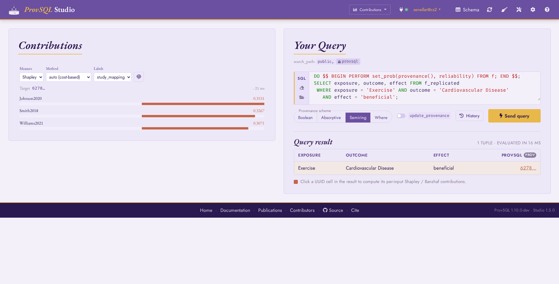
Contributions mode: Johnson2020, Smith2018, and Williams2021 ranked by Shapley value – the same numbers as Step 13, read off a heat-map. The Measure toggle switches to Banzhaf (Step 14).
Step 16: Arithmetic on Aggregate Results
ProvSQL tracks provenance through SQL aggregates: COUNT, SUM, and
similar produce aggregate tokens (agg_token) that record the underlying
contributions – and arithmetic (*, +…) over those aggregates stays
inside provenance: the result is itself an aggregate token whose circuit
combines the operand aggregates.
Compute a composite evidence weight per (exposure, outcome, effect) triple
combining how many studies report it (COUNT(*)) with the highest
reliability among them (MAX(reliability)):
SELECT exposure, outcome, effect,
       COUNT(*)           AS n_studies,
       MAX(reliability)   AS top_reliability,
       COUNT(*) * MAX(reliability) AS evidence_weight,
       (COUNT(*) * MAX(reliability))::NUMERIC AS evidence_weight_value
FROM f
GROUP BY exposure, outcome, effect
ORDER BY evidence_weight_value, exposure, outcome, effect;
Note
evidence_weight is an aggregate token: it can be inspected and
evaluated like any other provenance circuit, but it is not a plain
number. To get its value, cast it to NUMERIC as in
evidence_weight_value – the cast extracts the computed number at
the price of losing the provenance, making it ordinary SQL data
again (usable in ORDER BY, comparisons, further computation).
The group provenance – the token associated with each
(exposure, outcome, effect) triple – is unaffected and remains
available for probability_evaluate, shapley,
etc. on the group itself.