ProvSQL Studio
ProvSQL Studio is a Python-backed web UI for the ProvSQL extension. It runs as a separate package, connects to any PostgreSQL database with ProvSQL installed, and lets you inspect provenance interactively through four complementary modes:
Circuit mode renders the provenance directed acyclic graph (DAG) behind a result’s UUID or aggregate token, with frontier expansion, a node inspector, and on-the-fly semiring evaluation.
Contributions mode ranks the input tuples by their Shapley value or Banzhaf power index toward a chosen result tuple, as a heat-map of signed contribution bars.
Where mode highlights the source cells that contributed to each output value, against the live content of the provenance-tracked relations.
Notebook mode is a Jupyter-style notebook – SQL, Markdown, circuit and evaluation cells over a persistent database session – saved and loaded as standard
.ipynbfiles.
A schema panel, a configuration panel, and a mode-switcher round out the UI; all are described below. Throughout the UI, help icons deep-link into the relevant section of this manual. Like the extension, Studio is free, open-source software distributed under the MIT License.
Tip
Try it in your browser, no install: the same Studio UI, with
PostgreSQL and ProvSQL compiled to WebAssembly, runs entirely
client-side as the ProvSQL Playground at
provsql.org/playground/, on the
tutorial and case-study databases; a first visit opens the
interactive tutorial notebook. It needs a recent browser with
WebAssembly JSPI; the landing page lists current browser support.
Because the browser cannot launch external programs, the external
knowledge compilers and model counters, as well as graph-easy for
view_circuit, are not available there: probability is
computed with ProvSQL’s built-in methods, and everything else works.
Studio combines well with psql: bulk fixture loads
(psql -d mydb -f setup.sql) can go through psql before Studio
takes over, or live in the setup cells of a notebook (see
Notebook mode).
Installation
Studio targets Python ≥ 3.10. The released package is on PyPI:
pip install provsql-studio
Studio assumes the ProvSQL extension is already installed in the target database (see Getting ProvSQL) and is running at least the version listed under Compatibility.
For Studio developers, install from a local checkout in editable mode, so edits to the source take effect without reinstalling:
pip install -e ./studio
The Docker demonstration container ships a pre-installed Studio alongside the extension; see Docker Container.
Connecting
Launch Studio with a data source name (DSN):
provsql-studio --dsn postgresql://user@localhost:5432/mydb
If --dsn is omitted, Studio resolves the connection target in
this order:
The
DATABASE_URLenvironment variable, used as a DSN.libpq’s standard environment variables (
PGDATABASE,PGSERVICE,PGHOST…).Fallback to the
postgresmaintenance database on libpq’s default host (a local Unix socket on Linux and macOS,localhoston Windows). Studio then surfaces a banner inviting you to pick a real database from the in-page switcher.
The browser reaches the UI at http://127.0.0.1:8000/ (override
the bind address and port with --host and --port).
In-page connection editor
A plug icon () next to the connection-status dot in the top navigation
opens a pop-up panel where you can paste a DSN. Studio
probes the new DSN with SELECT 1 before swapping pools, so a typo
or wrong password leaves the existing connection up and surfaces the
PostgreSQL error inline. The status dot polls every 5 seconds; its
tooltip shows the active user@host:port endpoint.
Database switcher
Clicking the database name in the top nav lists every accessible database on the current server; pick one and the page reloads onto it. The query box is wiped on switch (the previous query rarely makes sense against a different database) but is pushed onto the history first, so Alt+↑ recovers it.
Two utility buttons sit nearby in the top nav: refreshes
Studio’s cached metadata (schema, provenance mappings, custom
semirings) after changes made outside the Studio session, and
empties the connected database, dropping every user
schema for a clean slate (the provsql extension survives).
Search path
Studio pins provsql at the end of the per-batch search_path
automatically, so the case-study idiom
SET search_path TO public, provsql; is unnecessary. The header
shows a lock chip for the pinned provsql; the rest of
search_path is editable under the Session group of the
Config panel (see Configuration).
Studio does not enforce a read-only PostgreSQL role: the query box
accepts arbitrary SQL, including DDL (CREATE TABLE), DML
(INSERT, UPDATE), and management helpers
(add_provenance, set_prob,
create_provenance_mapping).
Connect Studio with a role that has the privileges your workflow
expects.
Circuit mode
Circuit mode is the visual counterpart to view_circuit
and the programmatic walks via get_gate_type,
get_children, and identify_token. The query
runs unwrapped, so the provsql UUID column and any agg_token
cells appear in the result table as raw values; clicking one renders
its provenance DAG in the sidebar.
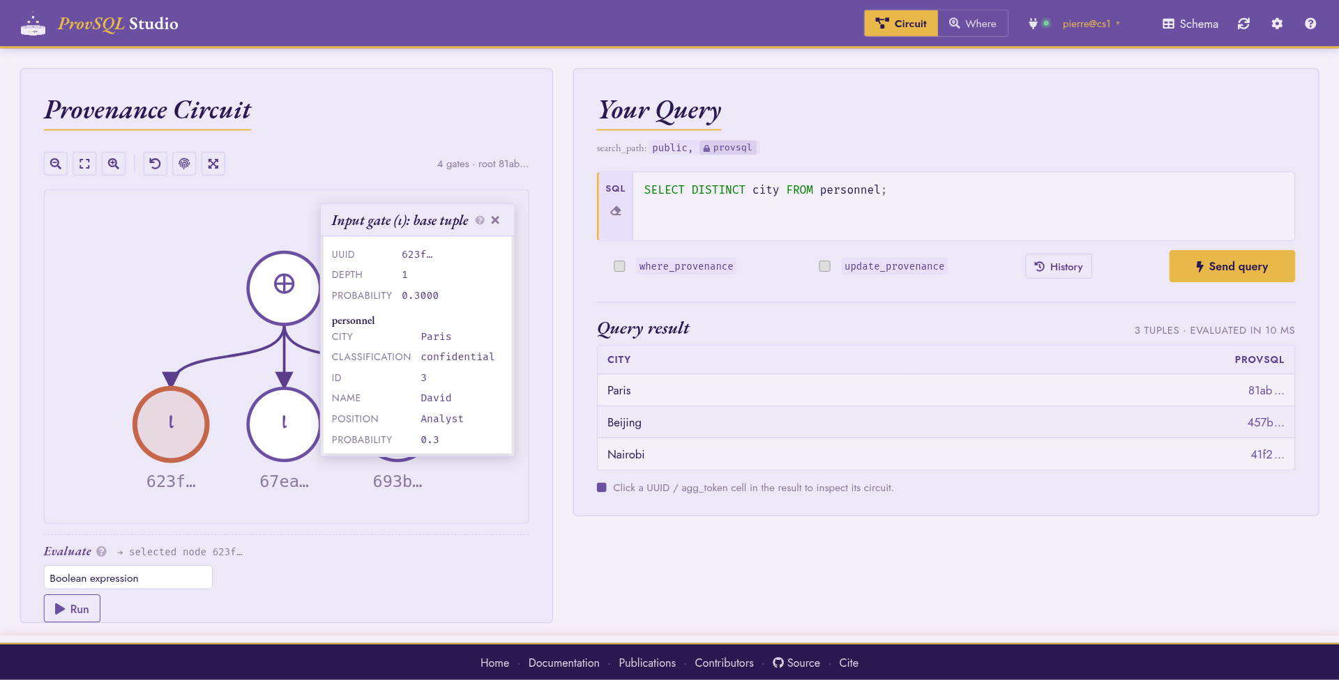
Circuit mode: a DISTINCT query renders a ⊕-rooted DAG.
Pinning an input gate opens the inspector with its metadata and
the stored probability, click-to-edit.
Hovering a node lights up its subtree; clicking pins it and opens the inspector panel. Drag a node to reposition it; the offset is preserved across frontier expansions and reset on every fresh circuit load. A Reset node positions toolbar button undoes all drag-to-move offsets at once. Wheel-to-zoom is supported on the canvas (with / zoom buttons in the toolbar), and a Fit to screen button resets zoom and pan. A Fullscreen toggle pins the canvas to the browser window (Esc exits), and a Show UUIDs toggle expands the abbreviated UUIDs – in the result table, on the canvas, and in the inspector – to their full form.
Query box
The query box is a syntax-highlighted SQL editor: PostgreSQL keywords, strings, comments, and identifiers are coloured inline.
Submit the current batch with Ctrl+Enter (or ⌘+Enter on
macOS) inside the query box, or by clicking the Send query button
next to it. While a batch is running, Send query gives way
to a Cancel button that interrupts the
statement in flight. Two gutter actions on the editor clear the query
box () and load a .sql file into it ().
Past queries are kept in a session history. Alt+↑ and Alt+↓ step through them in place; the History button opens a list view of recent queries to pick from.
The query box accepts multiple semicolon-separated statements;
Studio splits and runs them in a single transaction. Only the
last statement’s result is rendered in the result table;
preceding statements are useful for setup (SET,
CREATE TABLE, fixture INSERTs…) before the interesting
SELECT.
The result table is capped at Result rows (default 1000 rows,
tunable in Configuration). When more rows are available, the
result-table footer shows a (first 1000; more available) marker
so the truncation is explicit.
Each column header carries the column’s SQL type name as a tooltip, and
ProvSQL-significant columns get a small pill next to the column
name, mirroring the schema-panel pills described under
Schema panel: terracotta rv for
random_variable, terracotta agg for agg_token, and
purple prov for the row-provenance provsql column itself.
The pills make it obvious which result columns carry circuit
references (and are therefore clickable in Circuit mode) without
having to inspect the schema panel.
The prov pill is kind-aware: when the planner-side classifier
(provsql.classify_top_level, which
Studio enables automatically) certifies the result, the pill becomes
prov-tid or prov-bid accordingly; an OPAQUE result keeps
the bare prov label but in a muted tone so the lack of
certification is visible at a glance. Hovering the pill surfaces
the certified kind’s meaning plus the list of provenance-tracked
source relations the query touches, which is the same information
the underlying NOTICE carries.
Per-query toggles
A four-way Provenance scheme switch next to the query box selects which provenance behaviour the connection runs under for the next batch :
Semiring (default) : standard provenance tracking, no special configuration enabled. The resulting circuit accepts every compiled and custom semiring.
Where : sets
provsql.provenance = 'where', so the planner emitsprojectandeqgates that record the source cell of each output value (see Where-Provenance). Where mode (top nav) locks this position on, because the hover-to-trace surface needs the where-provenance gates ; in Circuit mode the choice is free.Boolean : sets
provsql.provenance = 'boolean', so the planner runs the safe-query rewriter and tags the resulting root with a Boolean-rewrite marker (see Probabilities). Only Boolean-faithful semirings will evaluate the resulting circuit ; the eval-strip semiring picker filters incompatible entries out when the root carries the marker.Absorptive : sets
provsql.provenance = 'absorptive', licensing constructions sound only for absorptive semirings – chiefly stopping a cyclic recursive query at its absorptive-value fixpoint (the minimal-paths semantics; see Network reliability on bounded-treewidth graphs) and the absorptive circuit simplifications. Only absorptive (and Boolean-rewrite-compatible) semirings then evaluate the circuit.
The selected scheme is session-sticky : it persists across
batches so two queries run with the same scheme without
re-toggling. An update_provenance (provsql.update_provenance)
checkbox next to the switch carries provenance through
INSERT, UPDATE, and DELETE statements (see
Data Modification Tracking) ; the checkbox is independent of the
scheme and freely user-controllable.
Both the scheme and the checkbox are sent to the server alongside each query.
Worked example
Ask for the distinct cities mentioned in personnel:
SELECT DISTINCT city FROM personnel;
The result table shows one row per city with a provsql UUID
column. Clicking a UUID cell renders the corresponding circuit: a
single ⊕ (plus) gate over the input gates of the underlying
personnel rows. Clicking a column header sorts the table by that
column (ascending, then descending on the next click; numeric columns
sort numerically, with blank cells sinking to the bottom). This works
on every Studio table, including the knowledge-compilation benchmark.
Frontier expansion
Studio caps each circuit fetch at the value of
--max-circuit-nodes (default 200, tunable in
Configuration). Nodes whose children were not fetched in the
current request carry a small gold + badge: clicking it requests
another breadth-first search (BFS) layer rooted at the frontier node
and merges it into the current scene. The cap is per-fetch, not per-scene, so a circuit
grows interactively as you expand the frontiers that interest you.
Inspector panel
Pinning a node opens the inspector. Each gate type (see
Inspecting the Circuit for the catalogue) renders a gate-specific
metadata block: function and result type for agg, left and right
attribute for eq, value for mulinput, relation id and
column list for input and update, and so on.
input and update gates additionally show the stored
probability: clicking the value swaps it for a number input, Enter
sends a set_prob to the server, Esc or clicking elsewhere cancels.
Out-of-range values and ProvSQL errors land inline.
A gate_assumed wrapper labelled 'boolean' (added by the
safe-query rewriter when the provenance class is 'boolean') is
rendered as a small B badge stamped on top of its child gate
rather than as a separate node, since structurally it is a marker
rather than a distinct operation; the load-time Boolean-only folds
stamp the same badge on the gates they rewrite. A wrapper labelled
'absorptive' (a recursive query truncated at the absorptive
value fixpoint, or compiled by the bounded-treewidth reachability
route), or the load-time absorptive folds, stamp an amber A
badge instead. Either badge narrows the evaluation strip’s semiring
menu to the options that are sound on the marked gate – only
absorptive semirings for a recursion root (including Tropical
(min-plus, nonnegative), which computes exact min-cost reachability
there), absorptive or Boolean-compatible ones for fold-marked gates.
A plus / times gate carrying the persisted d-DNNF
certificate (deterministic alternatives / decomposable conjunction
by construction – emitted by the bounded-treewidth reachability
route and the certified HAVING enumerations, see
Probabilities) is stamped with a green D badge; its
inspector states which property is certified. The certificate is
what routes probability_evaluate to the linear exact
independent method on these subcircuits.
The inversion-free certificate (a gate_annotation wrapper on a
certified result root, see Probabilities) is likewise elided
and rendered as a teal IF badge on its child. Its dashed ring
is drawn concentric outside the Boolean ring, so that on the rare
gate marked both ways the two rings stay distinguishable rather than
overlapping. Pinning that root shows the certificate header (atom / class counts)
and the variable-block order in the inspector. Pinning a certified
leaf surfaces its per-input order key (root value, secondary value,
factor – or the shared self-join guard) and its rank within the
shown scene in the inspector.
Semiring evaluation strip
Below the canvas, the semiring evaluation strip targets the pinned node (or, when no node is pinned, the root). The semiring select organises compiled entries into four sub-groups, with custom and “Other” entries below:
Compiled semirings
Boolean:
boolexpr,boolean.Lineage:
formula,how,why,which.formulapretty-prints the provenance circuit as a symbolic expression [Green et al., 2007];howis the same algebra in canonical![\mathbb{N}[X]](../_images/math/c6702caedfde7c46597c7b63ed37d7127165d138.svg) sum-of-products form, so two
semantically-equal circuits collapse to identical strings :
suitable for provenance-aware equivalence checks.
sum-of-products form, so two
semantically-equal circuits collapse to identical strings :
suitable for provenance-aware equivalence checks. whyandwhichare the set-valued projections.Numeric:
counting,tropical,viterbi,lukasiewicz. Łukasiewicz is the continuous-valued fuzzy logic on numeric values in![[0, 1]](../_images/math/3d075831ac3d404fd5808ee4d7b0b1091805368a.svg) ; for the discrete fuzzy /
trust shape on a user-defined enum lattice, see
; for the discrete fuzzy /
trust shape on a user-defined enum lattice, see maxminunder User-enum below.Intervals:
interval-union. One UI option backed by thesr_temporal,sr_interval_numandsr_interval_intkernels: the strip picks the right one from the selected mapping’s multirange type (tstzmultirange/nummultirange/int4multirange); requires PostgreSQL 14+. See Temporal Features for the interval-union algebra.User-enum:
minmaxandmaxmin. One UI option per shape, polymorphic over any user-defined PostgreSQL enum carrier (the bottom and top of the lattice come frompg_enum.enumsortorder).minmaxis the security shape (alternatives combine to enum-min, joins to enum-max);maxminis the discrete fuzzy / availability / trust shape (alternatives to enum-max, joins to enum-min). Backed bysr_minmaxandsr_maxminrespectively.
Custom semirings: any user-defined wrapper over
provenance_evaluatediscovered in the schema.Other:
probabilityandPROV-XML export. The probability method picker (see Probabilities) groups exact methods ((default),independent,possible-worlds,tree-decomposition,compilation), weighted model counting (wmc, with a tool picker), and approximate methods (monte-carlo,karp-luby). Two further exact methods appear only when the target’s structure admits them:inversion-freeon a root carrying an inversion-free certificate, andmobiuson a Möbius (μ) root. PROV-XML export usesto_provxml; see Provenance Export.
The mapping picker filters on the selected semiring’s expected value
type: only boolean-typed mappings appear under boolean, only
the numeric base types (smallint / integer / bigint /
numeric / real / double precision) under the numeric
group, only multirange-typed mappings under interval-union, and
only mappings whose value column is a user-defined enum
(pg_type.typtype = 'e') under minmax / maxmin.
Polymorphic entries (boolexpr, formula, how, why,
which) accept any mapping. boolexpr and PROV-XML export accept the
mapping as optional: with one, leaves are labelled by the mapping’s
value column; without one, leaves carry their gate UUID
(PROV-XML) or a bare x<id> placeholder (boolexpr). Custom-
semiring entries filter to mappings whose value type matches the
wrapper’s return type. Mismatches are surfaced before the round-trip
as (no compatible mappings : expected …) in the picker.
Run reports the result inline along with the runtime. For an
approximate method the strip also shows the (ε, δ) error bound ProvSQL
reports for that run: a relative error bound (the estimate is within a factor
1 ± ε of the true probability) for karp-luby and the weighted counters,
shown as relative error ≤ 10%, prob ≥ 95%; and an additive bound (a
Hoeffding absolute error,
https://en.wikipedia.org/wiki/Hoeffding%27s_inequality) for
monte-carlo, shown as ± 0.0136 absolute, prob ≥ 95%. The sample-based
methods also report the actual sample count (informative on the adaptive
(ε, δ) path, where ProvSQL derives it), e.g. …, 2,120 samples.
Clear wipes the result so a verbose Why or Formula output does
not obscure the canvas; Copy writes the just-rendered payload
(with full precision for probability, regardless of the rounded
display) to the clipboard.
The probability cell click-toggles between rounded (per the panel’s Probability decimals setting) and full double-precision; copies always carry the full-precision form.
The same evaluation picker also exposes the knowledge-compilation
pipeline, not as a side-effect of a probability run but as its own
standalone entries: a Knowledge compilation group offers the DIMACS
CNF (tseytin_cnf), the compiled d-D circuit
(compile_to_ddnnf_dot), the same d-D in NNF text form, and
the tree decomposition with its treewidth
(tree_decomposition_dot); the Probability group adds a
Probability benchmark that times every method (with a
per-method timeout, skipping unavailable tools). Selecting one and pressing
Run produces the artifact directly: the d-D circuit and the
tree decomposition take over the main canvas (a toolbar
back button restores the original provenance circuit), while the CNF and NNF
render as text panels. Compilers that are not installed on the server
are filtered out of the compiler picker (via tool_available).
See Knowledge Compilation for the full pipeline.
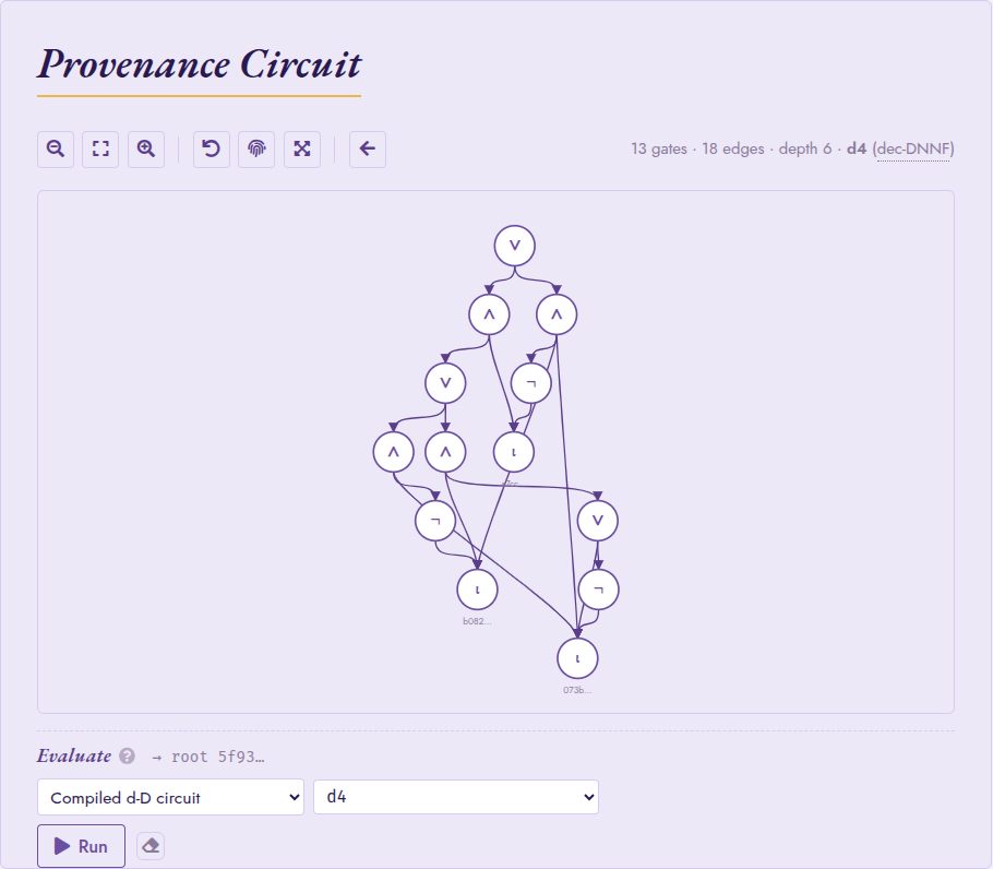
Knowledge compilation in Circuit mode: the provenance circuit of a
self-join, compiled to a d-DNNF by d4 (here 13 gates / 18 edges
/ depth 6). The canvas subtitle reports the compiled size and target
language; the back arrow in the toolbar restores the
original provenance circuit.
The d-DNNF and tree-decomposition canvases pin and inspect like the provenance circuit, with two refinements specific to those views:
In the tree-decomposition canvas, each bag is coloured by its index in the elimination order and clicking the bag focuses the inspector on its members. The inspector resolves each member’s source row (provenance UUID → table / row), so the user can trace back which tuple a given variable came from.
When a tree-decomposition bag or an internal d-DNNF gate (AND / OR / NOT) is pinned, the evaluation strip hides itself: those nodes are intermediate artifacts of the compilation, not roots of a probabilistic sub-circuit, so the usual semiring / probability surface does not apply.
When the pinned node is instead an agg_token or semimod gate
over random variables, the strip extends the moment / distribution-
profile / sample surface (otherwise offered on random_variable
leaves; see Continuous Distributions) to the aggregated value,
and hides the eval-strip options that do not apply to such a target.
Oversized circuits
When a top-level circuit fetch exceeds the cap, Studio shows a
structured banner instead of an error: This subgraph has 4,521
nodes; the cap is 200 (rendering at depth 4) followed by a
single-click Render at depth 1, then expand interactively button
when the depth-1 envelope itself fits under the cap. Wide-bound
circuits (for instance aggregations with high fan-in) leave the
button out rather than promising a render that will exceed the cap
again. The eval strip (above) still works against the unrendered
root: it operates on the token UUID, not the rendered DAG.
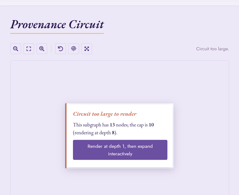
The actionable oversize-circuit banner: when a fetch exceeds the cap, Studio surfaces a single button to start at depth 1 and expand on demand.
Distribution profile panel
For nodes whose underlying gate is a scalar random-variable root
(gate_rv, gate_value in float8 mode, gate_arith,
gate_mixture), the eval strip exposes a Distribution profile
entry under the Distribution group. Running it returns
header stats (mean  and variance
  ),
an inline-SVG histogram of the sub-circuit’s distribution, a
PDF/CDF toggle, per-bar tooltips with
),
an inline-SVG histogram of the sub-circuit’s distribution, a
PDF/CDF toggle, per-bar tooltips with  markers, and
wheel-zoom on the value axis. The histogram is backed
server-side by
markers, and
wheel-zoom on the value axis. The histogram is backed
server-side by rv_histogram; the sample count comes
from provsql.rv_mc_samples and the seed from
provsql.monte_carlo_seed (both surfaced in the Config panel).
When the pinned node resolves to a recognised closed-form shape
the panel overlays the analytical PDF (or CDF, depending on the
toggle) on the histogram as a smooth terracotta curve, and
point masses as vertical stems capped by a small disc. The
overlay makes the simplifier’s analytical wins visible: when
2 * Exp(0.4) folds to Exp(0.2) the panel shows the
exact exponential decay curve over the MC-sampled bars, so the
user can verify by eye that the fold matched the distribution.
The recognised shapes are:
a bare
gate_rvof Normal / Uniform / Exponential / Erlang, optionally with a one-interval conditioning event – smooth curve;a Dirac (
provsql.as_random(c)) – single stem atc;a categorical (
provsql.categorical) – one stem per outcome, height proportional to its probability mass;a Bernoulli mixture (
provsql.mixture(p, X, Y)) over any recursively-matched shape – weighted sum of the per-arm curves, with Dirac / categorical arms contributing stems whose mass propagates through the Bernoulli weight.
Conditioning (a WHERE predicate, or any conditioning
provenance UUID) applies to every shape: bare-RV curves clip
to the conditioning interval and renormalise; mixture arms
truncate individually and the Bernoulli weight rebalances by
the ratio of arm masses; categorical outcomes outside the
interval are dropped and surviving masses renormalise to 1;
Diracs survive iff their value sits in the interval, and an
infeasible event raises a clean “conditioning event is
infeasible” error without running 100,000 wasted MC samples.
The curve is computed server-side by
rv_analytical_curves; shapes outside the closed-form
table (gate_arith composites of independent RVs that the
simplifier cannot fold, non-integer Erlang shapes) render
histogram-only without an overlay.
For pure-discrete shapes (a Dirac, a categorical, or a nested mixture whose every arm is one of those) the CDF mode draws a true staircase: horizontal flats joined by vertical jumps at each outcome, running from 0 at the chart’s left edge to 1 on the right.
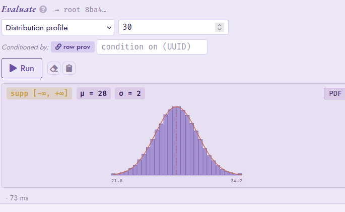
The Distribution profile eval-strip panel on a gate_rv
N(28, 2) leaf: header stats (support, ,
), an inline-SVG histogram with the analytical
PDF overlaid as a smooth terracotta curve, and a PDF/CDF
toggle on the right.
The same group hosts a Sample entry that draws raw samples
via rv_sample; the result renders as a collapsible
panel with a six-value inline preview and a “show full list”
expander. When the conditioning event’s acceptance
rate truncates the run below the requested n, the panel
surfaces an actionable hint pointing at provsql.rv_mc_samples.
The Moment entry on the same strip computes moment
or central_moment for a chosen k (raw vs central
toggle), and the Support entry returns the closed-form
support interval.
Conditioning and the row-prov auto-preset
The eval strip carries a Condition on text input that takes any provenance UUID, when populated, every distribution-shaped evaluation (profile, sample, moment, support) routes through the conditional path. Clicking a result-table cell auto-presets the field to the row’s provenance UUID, with a Conditioned by: row prov badge visible underneath the input. Clicking the active badge clears the conditioning and reverts to the unconditional answer; clicking the muted badge restores the row provenance. Manual edits stick within a row and reset on row navigation.
Combined with the distribution profile, this makes side-by-side comparison of unconditional vs conditional shape two clicks: pin the random variable, run Distribution profile unconditional, toggle the badge, run it conditional. The truncated closed-form table (Normal via Mills ratio, Uniform on the intersected support, Exponential by memorylessness) takes over when applicable; otherwise the panel reflects the rejection-sampling estimate at the configured budget.
Simplified-circuit rendering
Circuit mode honours the provsql.simplify_on_load setting
(see Configuration Reference and Continuous Distributions) and
renders the in-memory peephole-simplified graph via the
simplified_circuit_subgraph SRF. Toggling it in
the Config panel switches between the raw, gate-creation view
(useful when debugging RV constructors or the comparison-rewriter
path) and the simplified, evaluation-time view (what every
downstream consumer sees). Comparators decidable from the
propagated support (a Normal restricted to x > 2 reduces
trivially when shifted out of the support) collapse to Bernoulli
gate_input leaves before the canvas renders, so the visible
graph matches what the semiring evaluators and Monte-Carlo
sampler actually consume.
Contributions mode
Contributions mode answers a different question from Circuit mode: not
how a result tuple was derived, but how much each input tuple
mattered to it. It is the visual counterpart of the shapley
/ banzhaf family (see Shapley and Banzhaf Values), turning the bulk
shapley_all_vars / banzhaf_all_vars enumeration
into an interactive, ranked heat-map.
Queries are typed into the same Query box as in Circuit mode, under
the same Provenance scheme. Run a query, then click a result row’s
provsql cell to pin it as the target tuple: the contribution
of every input tuple toward that target is computed and drawn in the
sidebar. When the result has a single UUID-typed cell, it is pinned
automatically, as in Circuit mode.
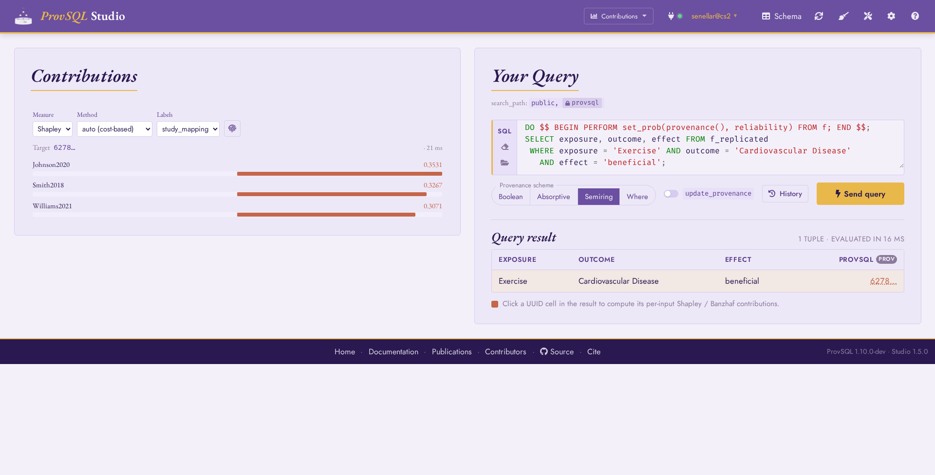
Contributions mode: the pinned target token at the top, then one signed contribution bar per input, ranked by magnitude.
Each bar diverges from a central baseline (positive contributions grow
right, negative ones – possible under monus-based or
conditioned circuits – grow left), scaled to the largest magnitude in
the set, with the numeric value alongside. The value is shown to the
configured number of decimals; click it to
expand it to full precision and copy that value to the clipboard. The
controls above the chart drive the computation:
Measure : Shapley (averaged over input orderings) or Banzhaf (averaged over coalitions). Both are computed in the expected probabilistic sense, so the Shapley values of all inputs sum to the target’s marginal probability.
Method : how the decision-diagram behind each value is built. auto cost-selects the cheapest route (
interpret-as-dd/tree-decomposition/compilation), reusing the probability chooser’s cost model; the named routes force one. compilation runs the external d-DNNF compiler chosen in the adjacent Compiler picker.Compiler : shown only for the compilation method, it lists the external d-DNNF compilers the server can reach (the same tool registry Probability evaluate draws on). In the Playground, where no compiler is bundled, the list is empty.
Labels : the provenance mapping whose
valuecolumn names the inputs (theON provenance = variablejoin). With source row selected instead, each input is resolved to its full tracked row (in table-column order) viaresolve_input; the bar shows the values and its tooltip names every column.
The Show full UUIDs toggle expands every abbreviated UUID (the target line, the result cells, and any unresolved input labels) to its full form, as in Circuit mode. The round-trip time of each computation is reported next to the target token, so the Method routes can be compared on cost.
Changing any control re-computes for the pinned target. A wide input relation can mint thousands of variables; the chart shows the top 200 by magnitude and reports the total when it truncates.
Where mode
Where mode is the visual counterpart to where_provenance
(see Where-Provenance). Queries are typed into the same
Query box as in Circuit mode. Where mode enables
provsql.provenance = 'where' on the connection and wraps every
SELECT so the result carries the where-provenance of each output
value. Hovering a result cell highlights the source cells (in
the sidebar) that contributed to it. No explicit
where_provenance call is required.
Where mode: source relations on the right; hovering a cell highlights the personnel rows that produced it.
The sidebar lists every provenance-tracked relation. Each panel
header reports its row count: personnel – 100 of ~50000 tuples
makes the per-relation cap explicit when a relation is too large to
materialise in full (default 100 rows, tunable in
Configuration). The Input gates only toggle (default on)
hides relations whose first provsql token is not an input
gate, so derived materialisations do not crowd the panel.
Each result row gets a Circuit button that switches to Circuit mode and pre-loads the provenance DAG of that row’s token, and a Contributions button that switches to Contributions mode and pins the same token; see Mode-switching.
Worked example
Ask for the people listed in Paris:
SELECT * FROM personnel WHERE city = 'Paris';
Each output cell becomes hover-aware: hovering name,
classification, or city lights up the matching cells in the
personnel panel of the sidebar.
Wrap-fallback notice
If a Where-mode query touches no provenance-tracked relation, Studio
silently drops the wrap and surfaces an INFO banner instead of
raising. This is the right default for case-study scripts that do
bulk setup before the first interesting SELECT.
Notebook mode
Notebook mode is a Jupyter-style notebook over your ProvSQL database:
an ordered list of cells – SQL, Markdown, circuit snapshots, semiring
evaluations – executed against a persistent database session (the
kernel) and saved as a standard .ipynb file. It is the right
mode for narrated, replayable analyses: the bundled tutorial and case
studies (see Example notebooks) are notebooks.
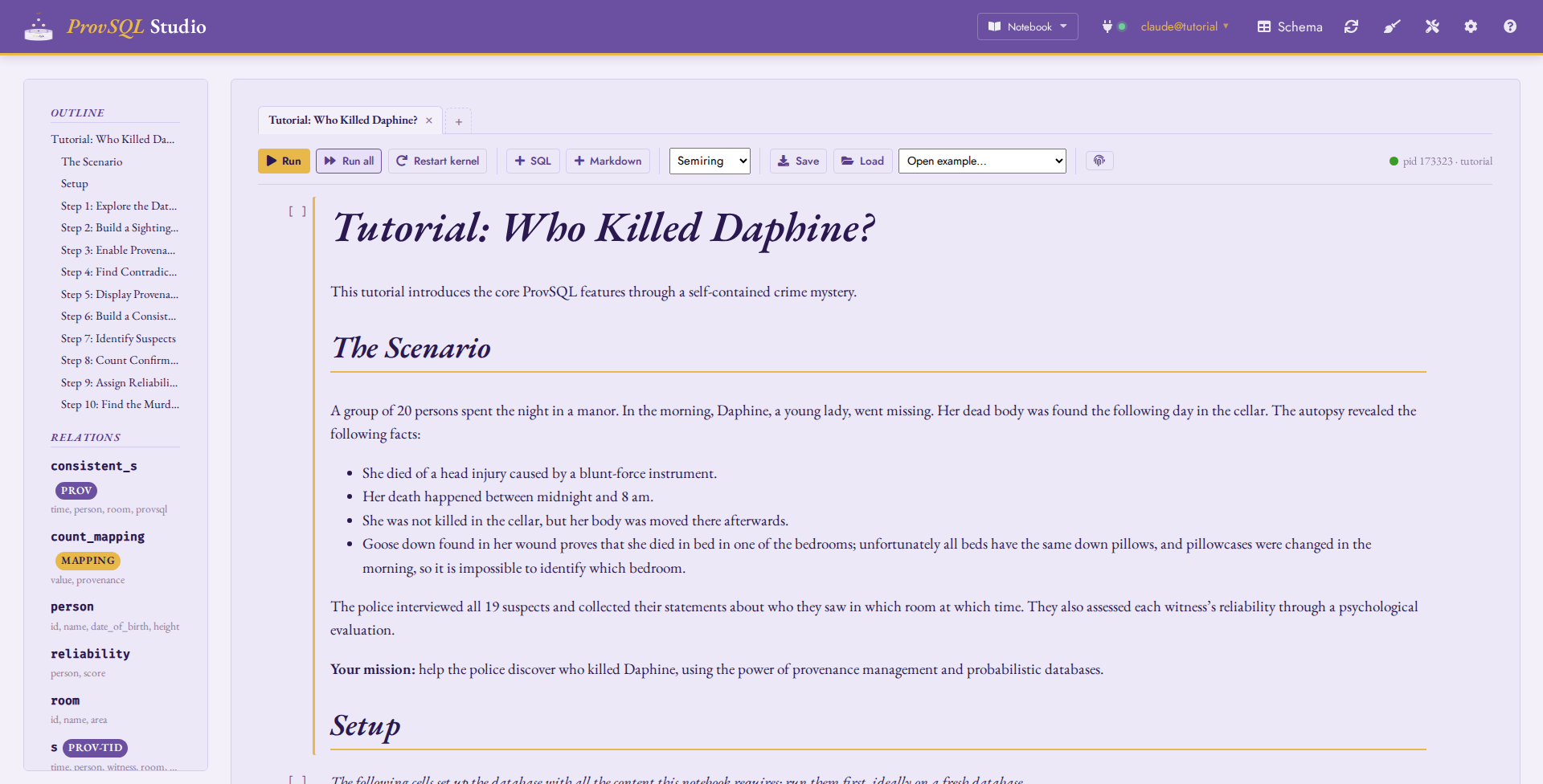
Notebook mode with the bundled tutorial open: the tab bar (one tab per notebook), the toolbar with the kernel chip, and the compact outline/relations sidebar.
Cells and the kernel
SQL cells run on the notebook’s kernel: a dedicated database
session that persists across cells, so temporary tables, SET
commands, and prepared statements made by one cell are visible to the
next – the Jupyter state model, with the database session playing the
part of the Python interpreter. Each cell executes in its own
transaction: a failed cell rolls back cleanly (the error lands in the
cell’s output) while previously committed cells persist. Execution
counters ([1], [2], …) track what ran on the current kernel,
and results render through the same table renderer as the query box –
provenance pills, clickable UUID cells and all.
The kernel starts lazily on the first run and its chip in the toolbar
shows the backend pid and database. Run runs the
selected cell; Run all executes the
cells top to bottom; Interrupt cancels the statement in
flight; Restart kernel discards the session (temporary
tables and session SET s are lost, counters reset), which is the
clean-slate button when state has drifted. Idle kernels are dropped
server-side after a timeout, and a connection switch drops them all;
the front-end simply starts a fresh kernel on the next run.
The toolbar also appends fresh cells ( SQL / Markdown) and, as in Circuit mode, expands abbreviated UUIDs in cell results to their full form (). Each cell carries its own run button and an action row: move it up / down ( / ), delete it (), insert a SQL () or Markdown () cell below, plus the per-cell scheme chip and Circuit-mode jump described below.
Markdown cells render GitHub-flavoured Markdown; fenced code
blocks tagged sql get the same syntax highlighting as the SQL
editors. Double-click (or press Enter) to edit, click away (or
Esc) to render.
Keyboard shortcuts
The keymap follows Jupyter’s two-mode model: command mode acts on the selected cell (highlighted border), edit mode types into it.
Key |
Action |
|---|---|
Enter / Esc |
Enter / leave edit mode on the selected cell. |
Ctrl+Enter |
Run the cell (render, for a Markdown cell), stay on it. |
Shift+Enter |
Run, then select the next cell; at the last cell, create a fresh SQL cell below and edit it. |
Alt+Enter |
Run, then insert a fresh SQL cell below and edit it. |
a / b |
Insert a SQL cell above / below. |
d d / z |
Delete the selected cell / undo the deletion. |
m / y |
Convert to Markdown / back to SQL. A non-empty SQL source is
wrapped in an |
j / k (or arrows) |
Select the next / previous cell. |
Circuit and evaluation cells
Clicking a provenance UUID in a result inserts a circuit cell below the query: a snapshot of the provenance DAG behind that token, painted with the same gate glyphs as Circuit mode (no depth control – the fetch is capped like Circuit mode’s initial render). Clicking a different UUID retargets the same cell, and re-fetches the snapshot against the live circuit; the Circuit mode button jumps to the full canvas (frontier expansion, inspector, evaluation strip) preloaded with the token.
For a plain provenance token, the circuit cell offers Evaluate, which inserts an evaluation cell: a compiled semiring or probability method, optional free-text arguments and provenance mapping, run against the cell’s token. The invocation and its result are saved with the notebook, so a loaded notebook shows its evaluations without recomputing them. (Aggregate and random-variable tokens get no Evaluate button: their dedicated dispatch – distribution profiles, moments, aggregate inspection – lives in Circuit mode, one jump away.)
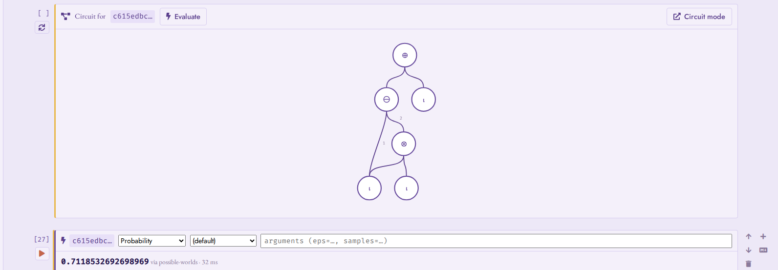
A circuit cell (one suspect’s provenance in the tutorial) and its evaluation cell: probability/exact on the pinned token.
Provenance scheme
The toolbar’s Provenance scheme selector is the notebook’s default (the same three-way switch as the query box, see Per-query toggles); each SQL cell can override it with the small scheme chip in its actions, cycled per cell and honoured at run time. Per-cell overrides are what make mixed notebooks work – e.g. one recursive-CTE cell running under the Boolean scheme inside an otherwise standard-provenance notebook.
Tabs and database bindings
A notebook is not the whole program: it runs against a database
whose state persists beyond it. Every notebook is therefore bound
to the database it was authored against (recorded in the .ipynb
metadata – the name only, never credentials), and the tab bar shows
one tab per open notebook, named after its first level-1 Markdown
heading. Loading a notebook always opens a new tab, bound per its
metadata.
When a tab’s binding differs from the live connection, a banner says so and offers the three sensible moves – switch the connection to the bound database, create it if it does not exist (the scratch-database escape hatch for hermetic runs), or rebind the notebook to the current database. Nothing switches silently.

The binding banner: this notebook expects cs1 but the
connection is on tutorial.
Saving, loading, autosave
Save downloads the notebook as an nbformat-v4 .ipynb
– directly openable in Jupyter-aware tooling. Cell outputs are
included with standard MIME fallbacks (HTML tables, self-contained
SVG circuit snapshots, plain-text evaluation results), so GitHub and
nbviewer render a saved notebook as a readable static document;
Studio itself re-renders from richer payloads stored alongside under
application/vnd.provsql.* keys. Load opens an
.ipynb in a new tab; it also accepts a .sql file (a fixture
script, a pg_dump dump…), appended to the current notebook as one
ready-to-run SQL cell. Between saves, every tab autosaves to the
browser’s local storage, surviving reloads and mode switches.
Example notebooks
The Open example… menu lists the bundled notebooks: this
manual’s tutorial and case studies, generated from the same sources as
the chapters you are reading. Each is self-establishing – it opens
with idempotent setup cells (schema, data, add_provenance) – so
running it top to bottom on a fresh database reproduces the whole
study from one file: open the example, let the binding banner create
the bound database if it does not exist yet (see Tabs and database
bindings), and press Run all. The
/notebook?nb=<name> deep link opens an example directly.
Notebook mode in the Playground
Notebook mode works in the Playground, with
one caveat: the in-browser PostgreSQL has a single session, shared by
every notebook tab’s kernel and by the other API calls. Kernel state
is therefore visible across tabs, and restarting any kernel (mapped
onto DISCARD ALL) resets them all. The binding banner’s
database-creation action works there too, and
?nb=<name> deep links open the bundled examples –
e.g. provsql.org/playground/?nb=tutorial.
Schema panel
A Schema button in the top nav opens a
searchable pop-up panel listing every SELECT-able relation. Each gets one of two relation-level
pills:
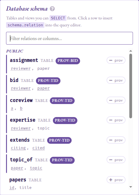
Schema panel: TID and BID sub-pills annotate each provenance-tracked
relation; primary-key columns are solid-underlined and repair_key
(BID) grouping keys dotted-underlined.
prov (purple) on a relation whose
provsqlcolumn is injected by the planner: provenance tracking is active. The pill is sub-classified by the relation’s certified kind (see Probabilities for the TID vs BID model) : PROV-TID for tuple-independent tables registered viaadd_provenance, PROV-BID for block-independent tables registered viarepair_key, and a bare prov in a muted tone for relations whose kind is opaque. This is the same classification the safe-query rewriter consults to decide whether a query is in scope for the'boolean'provenance class.mapping (gold) on a relation shaped
(value <T>, provenance uuid), including views fromcreate_provenance_mapping_view. The two pills are mutually exclusive: a mapping view that also carries a planner- injectedprovsqlcolumn is classified as mapping (the more specific category).
Clicking a relation row (or focusing it and pressing Enter / Space)
replaces the query box with a ready-to-run
SELECT * FROM <relation>; so the inspected table is one click
away from being queried.
Columns whose type is one of ProvSQL’s circuit-bearing types
carry their own terracotta pill next to the column name:
rv for random_variable (operators rewrite into
gate_cmp / gate_arith; see
Continuous Distributions) and agg for agg_token
(each value is a circuit root with a running aggregate value).
Key columns are underlined, following the relational-schema
convention: a solid underline marks a primary-key column, and a
dotted underline marks a repair_key (BID) grouping key, the
attribute whose value defines a block of mutually-exclusive rows (see
the TID vs BID model in Probabilities).
On a tracked table, each column is a click target that prefills
SELECT create_provenance_mapping('<table>_<col>_mapping',
'<schema>.<table>', '<col>');
into the query box, so a fresh
mapping is two clicks away. The click affordance is suppressed
on rv and agg columns, since their values are circuit
references rather than scalars and a mapping built from them
would not label input gates meaningfully.
On any provenance-eligible plain table, prov and
prov action chips prefill SELECT add_provenance(...)
/ SELECT remove_provenance(...). They are hidden on views
(regular and materialised) and on foreign tables, since the
underlying ALTER TABLE ADD COLUMN does not work on those
relation kinds, and on mappings.
Configuration
The Config panel groups its options into four sections:
Provenance mirrors the user-level configuration parameters documented in Configuration Reference:
provsql.active,provsql.verbose_level, andprovsql.tool_search_path.provsql.tool_search_pathis superuser-only (see Configuration Reference); when Studio is connected as a non-superuser role, its field is shown read-only and labelled (admin-managed), reflecting the value an administrator pinned (or the server’s defaultPATH) rather than letting an edit silently have no effect.provsql.provenanceandprovsql.update_provenancelive next to the query box instead (see Per-query toggles), since they are typically flipped per query rather than per session. Studio also forcesprovsql.aggtoken_text_as_uuid = onfor the whole session: clickableagg_tokencells in the result table need that.Probabilities gathers the GUCs that steer probability and random-variable evaluation:
provsql.simplify_on_load,provsql.monte_carlo_seed,provsql.rv_mc_samples(all documented in Configuration Reference), and aprovsql.fallback_compilerdropdown selecting the d-DNNF compilermakeDDfalls back to (see Knowledge Compilation), its choices validated against the compilers resolvable on the server.Session wraps the per-request session state: the
statement_timeoutapplied to every batch, and the visible part ofsearch_path(provsqlis always pinned at the end).Display limits holds the size knobs: Max circuit depth (the BFS depth cap on the initial fetch), Nodes per fetch (the per-fetch node cap), Sidebar rows per relation (per-relation row cap in the Where-mode sidebar), Result rows (row cap on the result table), and Probability decimals (number of decimals in the eval-strip’s probability display).
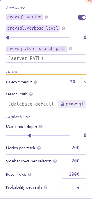
The Config panel: four section headings above the per-row options.
All values persist on disk in provsql-studio/config.json under
the platform’s user-config directory, and survive a Studio restart:
Linux:
$XDG_CONFIG_HOME/provsql-studio/(defaults to~/.config/provsql-studio/).macOS:
~/Library/Application Support/provsql-studio/.Windows:
%APPDATA%\provsql-studio\(typicallyC:\Users\<user>\AppData\Roaming\provsql-studio\).
Each option is also exposed on the CLI as a flag
(--statement-timeout, --max-sidebar-rows, --max-result-rows,
--max-circuit-nodes, --search-path, --tool-search-path);
the CLI wins on startup, the panel writes back to the JSON.
Tools panel
A tools button (the wrench-and-screwdriver icon, ) in the top nav,
left of the Config cog (), opens the external-tool registry –
the same provsql.tools
catalog the compilation and weighted-counting dropdowns draw from (see
External-Tool Registry).
Tools are grouped by operation (Compilation, Weighted counting,
Rendering). Each row shows a tool’s availability (a green dot when its binary
and dependencies resolve on the backend’s PATH, or, for a socket server,
when its endpoint is configured), its name, a cli / kcmcp badge, and
its endpoint or executable.
A superuser may manage the registry in place: edit a tool’s preference
(higher is selected first), toggle it on or off, edit it (the
pencil reopens the form pre-filled), or unregister it (the
cross). Register a tool opens the same form. Picking the Kind swaps the relevant fields: a
cli tool takes an executable and a command template; a kcmcp tool (a
warm KCMCP server) takes a Connection –
either Managed (ProvSQL launches and supervises it via
provsql.kcmcp_server) or an Endpoint address
(unix:/path or host:port). The input formats, output format, and
parser are offered as the values that make sense for the chosen operation.
The registry’s mutators are superuser-only, so a non-superuser session sees
the panel read-only.
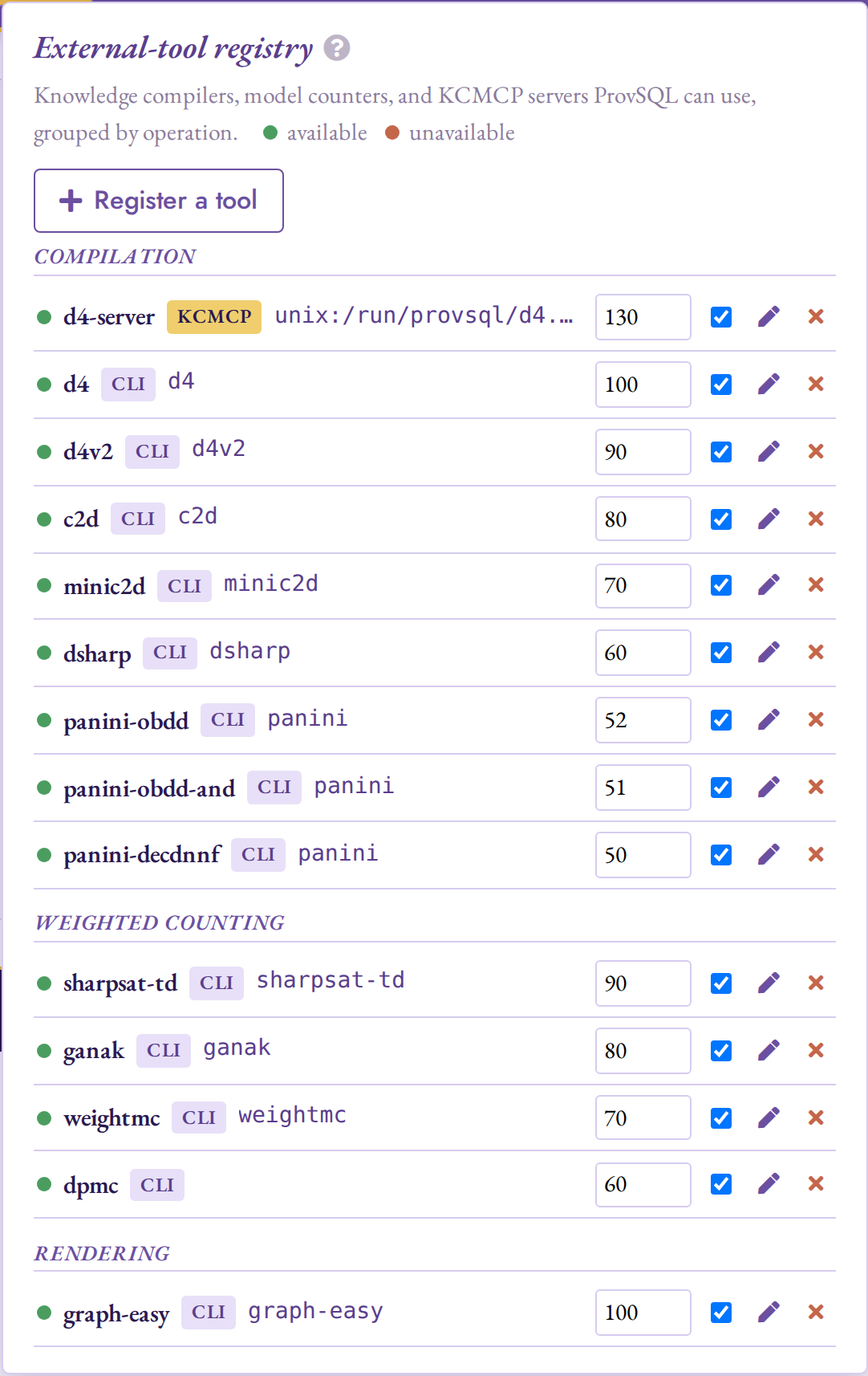
The Tools panel: the registry grouped by operation, each tool with its
availability, kind, preference, enable toggle, and edit / unregister
actions (here a kcmcp compile server at the top of Compilation).
Mode-switching
The mode tabs in the top nav switch between
Where, Circuit, and Notebook. A switch carries the current SQL forward via
sessionStorage (in Notebook mode, the selected cell’s SQL); it
auto-replays only when the user just ran the query, so unrun drafts
and plain reloads never auto-execute (important for side-effecting
statements like add_provenance).
In Where mode, every result row gets a Circuit button that switches to Circuit mode and pre-loads the circuit for that row’s provenance UUID, so a hover-and-trace exploration can cross over to the DAG without retyping the query. In Notebook mode, the per-cell open in Circuit mode action and the circuit cells’ Circuit mode button do the same; switching back returns to the same notebook, selection and scroll position included.
Limitations
Per-fetch circuit cap, not per-scene:
--max-circuit-nodesbounds each fetch independently, so a scene assembled by repeated frontier expansions can exceed the cap. This is intentional: the cap exists to keep the browser responsive on initial render, not to prevent drilling deep where you want to.Verbose semiring outputs are unbounded:
formula,how,why,which, andPROV-XML exportcan return multi-megabyte strings on large circuits. Compute time is bounded bystatement_timeout; output size is not. Use Clear after a bulky run, or evaluate against a pinned subnode to scope the output.
Compatibility
Studio’s version stream is independent of the extension’s. Studio
is released on PyPI as provsql-studio from studio-vX.Y.Z
git tags; the extension is released on PGXN as provsql from
vX.Y.Z git tags. Each Studio release lists a minimum required
extension version.
Studio |
ProvSQL extension |
Notes |
|---|---|---|
|
|
First public release. Requires |
|
|
Adds renderers for the continuous-distribution gate
family ( |
|
|
Adds the three-way Provenance scheme selector
(Semiring / Where / Boolean), the B badge on
|
|
|
Adds the knowledge-compilation strip (the DIMACS CNF with its
variable-to-source-tuple mapping, the compiled d-DNNF and
tree-decomposition canvases, the |
|
|
Adds the Tools panel: an in-app view of
the Also renders the inversion-free certificate: a teal IF
badge on a certified result root (coexisting with the Boolean
B badge), with the certificate header and variable-block
order in the inspector and the per-input order key plus rank on
certified leaves, and offers the |
|
|
Adds Notebook mode: a Jupyter-style
notebook (SQL / Markdown / circuit-snapshot / evaluation cells)
over a pinned kernel session, with the Jupyter keymap, per-cell
provenance-scheme overrides, tabs as database bindings,
|
|
|
Adds Contributions mode
(per-input Shapley / Banzhaf bars, over
|
When the installed extension predates this minimum, Studio’s startup
check prints the mismatch and exits. Pass --ignore-version to
override the check, for instance when running against a development
branch.